Postdoctoral Research Scientist Machine Learning, Department of Computer Science Mailing Address: Mail Code 0401 1214 Amsterdam Ave. New York, NY 10027 Location: Office: 612 Schapiro Center (CEPSR) Email: delbert@cs.columbia.edu Telephone: +1·212·939·7124

Latest Research: Perfect Graphs for Efficient MAP Inference
Downloads: fast and simple isperfect.c code  | all connected perfect graphs with {5,6,7,8,9,10} nodes | findholeofsizeD.m (large graphs) | findmaxcliques.m | isconnected.m

Graphical models have become an indispensible tool in machine learning and applied statistics for representing networks of variables and probability distributions describing their interactions. Recovering the maximum a posteriori (MAP) configuration of random variables in a graphical model is an important problem with applications ranging from protein folding to image processing. The task of finding the optimal MAP configuration has been shown to be NP-hard in general (Shimony, 1994), and has been well studied from several different perspectives, including message-passing algorithms (Pearl, 1988), linear programming relaxations (Taskar et al., 2004), and max-flow/min-cut frameworks (Greig et al., 1989). This work uses recent advances in the theory of perfect graphs to outline situations where provably-optimal solutions are possible to find with efficient algorithms in P, and provides several useful applications of this result.

Consider an undirected graph, G=(V,E) with n vertices V={v₁,...,v_n} and edges E: V×V$ →{0,1}.  Such a graph is perfect if every induced subgraph has chromatic number equal to its clique number. Perfect graphs originated with work by Claude Berge (1963); a graph is Berge if it and its complement contains no odd holes (i.e., no chordless cycles of length 5, 7, 9,..., etc.).  It is fairly straightforward to show that all perfect graphs are Berge, but the converse is not obvious; work in (Chudnovsky et al., 2006) enumerates the entire family of Berge graphs and shows that all family members are perfect.

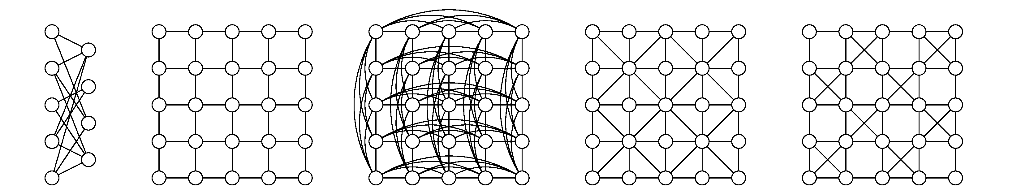
Some examples of perfect graphs are shown above.  Perfect graphs have remarkable computational properties in that often-intractable problems such as graph coloring, finding the size of the maximal clique, and maximum independent set can be found in polynomial time.

A Markov random field (MRF) is an undirected graphical model used to represent the factorization of a probability distribution. A nand Markov random field (NMRF) is a specific type of MRF whereby edges in the underlying graph represent pairwise nand relationships between binary variables represented by each graph vertex. There are also singleton weights, w, associated with each vertex.  As described in (Jebara, 2009), any MRF is efficiently convertible into a binary NMRF in time and space proportional to the number of variable configurations in maximal cliques.  Finding the MAP configuration of an NMRF is NP-hard in general but due to work by Lovász (1972) and Chvátal (1975) it can be done in polynomial time for perfect graphs.

There are several practical applications which are readily described by a perfect NMRF, including:
• Ising grid models have a rich history in statistical physics and are widely used in image-processing. Such graphs frequently appear similar to the sample graph above, and MAP solutions are typically found using graph cut algorithms based on reformulation as min-cut/max-flow problems (Greig et al., 1989).  It has been shown that graphs whose potentials are exclusively submodular are solvable in polynomial time (Kolmogorov et al., 2004), but the class of perfect graphs is more general and leads to provably-optimal solutions of some non-submodular energy functions using message-passing techniques such as MPLP.
• Bipartite matching (Bayati et al., 2005) and b-matching (Huang et al., 2007) are fundamental computer science problems that increasingly play important roles in Internet search applications. They are traditionally solved with using an inefficient albeit polynomial-time algorithm but more recent work has focussed on light-weight belief-propagation solutions and optimality guarantees. These problems are roughly expressed using line graphs of bipartite graphs (Rook's graphs) as shown in the previous Figure.
• Affinity propagation clustering (Frey et al., 2007), an algorithm that clusters data by identifying a subset of representative exemplars using loopy belief propagation. For some useful cases of affinity propagation which involve decisions between a small number of candidate exemplars, the problem becomes a perfect graph and provably-exact solutions can be found in polynomial time.

Thesis Research: Affinity Propagation

Here is my Ph.D. thesis, Affinity Propagation: Clustering Data by Passing Messages (smaller viewable PDF, large printable ZIP)

How would you identify a small number of face images that together accurately represent a data set of face images? How would you identify a small number of sentences that accurately reflect the content of a document? How would you identify a small number of cities that are most easily accessible from all other cities by commercial airline? How would you identify segments of DNA that reflect the expression properties of genes? Data centers, or exemplars, are traditionally found by randomly choosing an initial subset of data points and then iteratively refining it, but this only works well if that initial choice is close to a good solution. Affinity propagation is a new algorithm that takes as input measures of similarity between pairs of data points and simultaneously considers all data points as potential exemplars. Real-valued messages are exchanged between data points until a high-quality set of exemplars and corresponding clusters gradually emerges. We have used affinity propagation to solve a variety of clustering problems and we found that it uniformly found clusters with much lower error than those found by other methods, and it did so in less than one-hundredth the amount of time. Because of its simplicity, general applicability, and performance, we believe affinity propagation will prove to be of broad value in science and engineering.

The following animated visualization shows affinity propagation gradually identifying three exemplars among a small set of two-dimensional data points:

For more information, see http://www.psi.toronto.edu/affinitypropagation.

Earlier Research: Probabilistic Sparse Matrix Factorization

We propose a new method of finding sparse matrix factorizations employing probabilistic inference techniques, and apply them to discover structures underlying gene expression data.

Given a data matrix XÎÂ^G×T, containing G T-dimensional data points, we perform matrix factorization (X»Y·Z).  Specifically, we find a matrix of hidden factors (or causes), ZÎÂ^C×T, and a factor loading matrix, YÎÂ^G×C, under a structural sparseness constraint that each row of Y contains at most N (of C possible) non-zero entries.  Intuitively, this corresponds to explaining each row-vector of X as a linear combination (weighted by the corresponding row in Y) of a small subset of factors (causes) given by rows of Z.  Note that this framework includes simple clustering (N=1) and ordinary low-rank approximation (N=C) as special cases.

We construct a probability model presuming Gaussian sensor noise in X (i.e. X=Y·Z+noise) and uniformly distributed factor assignments.  We utilize a factorized variational method to perform tractable inference on the latent variables, and also account for noise in the factor matrix (Z) and uncertainty in assigning factors (Y).  We explore several different factorization depths to allow a tradeoff between increased model accuracy and decreased computational complexity.

Figure: Probabilistic Sparse Matrix Factorization of a 22709×55 gene expression array
Click for animation (1.2 MB)

We apply our algorithm to mouse gene expression data from the Hughes Lab, as shown in the figure above.  We show a data set of G=22709 gene expression profiles (expressed across T=55 tissues) approximated by linear combinations of at most N=3 (of a possible C=50) hidden transcription factor profiles.  Experimental results demonstrate that our method can identify genetic functional categories with higher statistical significance than the method currently in greatest use, hierarchical agglomerative clustering.

References:

Frey, B.J. and Dueck, D. (2008)
Affinity propagation and the vertex substitution heuristic. Science
319, 726d.
Dueck, D., Frey, B.J., Jojic, N. and Jojic, V. (2008)
Constructing Treatment Portfolios Using Affinity Propagation. To appear at
International Conference on Research in Computational Molecular Biology
(RECOMB), 30/03/2008 – 02/04/2008, Singapore.
Dueck, D. and Frey, B.J. (2007)
Non-metric affinity propagation for unsupervised image categorization.
IEEE International Conference on Computer Vision (ICCV).
Frey, B.J. and Dueck, D. (2007)
Clustering by Passing Messages Between Data Points. Science 315:
972–976.
Frey, B.J. and Dueck, D. (2006) Mixture modeling by Affinity Propagation.
Neural
Information Processing Systems. 18: 379–386.
Dueck, D., Morris, Q., and Frey, B. (2005)
Multi-way clustering of microarray data using probabilistic sparse matrix
factorization. Presented at the 13th Annual International conference on
Intelligent Systems for Molecular Biology (ISMB 2005).
Dueck, D., Huang, J., Morris, Q.D., and Frey, B. (2004)
Iterative Analysis of Microarray Data. 42nd Annual Allerton Conference on
Communication, Control, and Computing. (oral presentation 30/09/2004)
Dueck, D. (2004)
Probabilistic Sparse Matrix Factorization. Third Annual Information
Processing Workshop, Toronto, Canada (orally presented 11/08/2004)
Dueck, D. and Frey, B. (2004)
Probabilistic Sparse Matrix Factorization. University of Toronto
Technical Report PSI-2004-23.
MATLAB PSMF code