Rank Constraints for Recognition

If the image to image homography is affine, the transformation matrix has 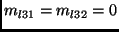$m_{l31} = m_{l32} = 0$ and $m_{l33} = 1$. The transformation can be expressed in terms of inhomogeneous coordinates as

$${\bf x}^l[i] = {\bf A}_l{\bf x}^0[i] + {\bf b}_l$$ (3)

where ${\bf x}^l[i]$ is the inhomogeneous representation of the $i$th point on the contour in view $l$, ${\bf A}_l$ is the upper $2\times 2$ minor of ${\bf M}_l$ and ${\bf b}_l$ is the upper two elements of the last column of ${\bf M}_l$.

The above expression is valid for the scenarios when correspondence between points across views is known. However in practice, correspondence is rarely available. In case correspondence information is not available, Equation 3 assumes the form

$${\bf x}^l[i] = {\bf A}_l{\bf x}^0[i+\lambda_l] + {\bf b}_l$$

where shifting ${\bf x}^0$ by $\lambda_l$ would align the corresponding points of ${\bf x}^0$ and ${\bf x}^l$. The frequency domain representation can be given by

$${\bf X}^l[k] = {\bf A}_l{\bf X}^0[k] \exp({\frac{j 2 \pi \lambda_l k}{N}}),\;\; 0 < k < N$$ (4)

if the ${\bf b}$ term is eliminated by omitting the $k = 0$ term in the Fourier domain.