We have now localized a set of possible candidates for objects of
interest (balls and pockets). To recognize and classify these objects,
we propose the use of color models. We train a set of probabilistic
color models for the pockets and the balls (cue ball, 8-ball, the
seven striped balls and the seven solid balls). We also train models of
other objects that might appear in the image as false alarms: a color
model of the pool cue and the player's hand. This process is identical
to the color modeling used for the table and we obtain a total of 20
models which have a form similar to
Equation ![]() . We shall refer to these models as
. We shall refer to these models as
![]() .
.
Figure ![]() and Figure
and Figure ![]() show the color
modeling process for the solid red ball and the striped orange
ball. For each model, we begin with a distribution of pixels in RGB
space as shown in Figure
show the color
modeling process for the solid red ball and the striped orange
ball. For each model, we begin with a distribution of pixels in RGB
space as shown in Figure ![]() (a) and
Figure
(a) and
Figure ![]() (a). These sets of 3 dimensional RGB vectors
are labeled
(a). These sets of 3 dimensional RGB vectors
are labeled ![]() . For each
. For each ![]() we compute a
model
we compute a
model ![]() when we first train the system.
when we first train the system.
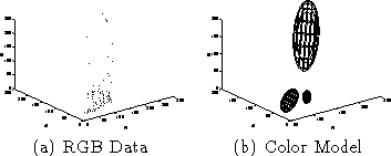
Figure: The Solid Red Ball (Trained)
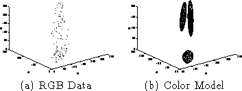
Figure: The Striped Orange Ball (Trained)
Next we apply all 20 color models to examine each of the possible
candidate symmetry peaks. Around each peak, we collect a small window
of pixels. All non-table pixels (i.e. the ones that did not match the
table's color model) are collected to form a distribution of RGB data
similar to the one in Figure ![]() (a). This test
distribution will be called
(a). This test
distribution will be called ![]() . We form a single Gaussian color
model (because EM with multiple Gaussians would be too slow to compute
online). This model, shown in Figure
. We form a single Gaussian color
model (because EM with multiple Gaussians would be too slow to compute
online). This model, shown in Figure ![]() (b), is
called
(b), is
called ![]() .
.
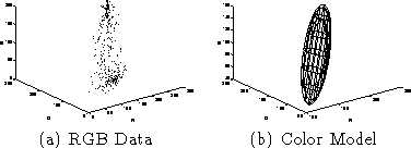
Figure: The Test Object (Orange Striped Ball)
To classify our test distribution ![]() we use a common distance
metric between probabilistic models. This metric is the
Kullback-Liebler divergence [4]
we use a common distance
metric between probabilistic models. This metric is the
Kullback-Liebler divergence [4] ![]() . By measuring the 'distance' between
test data
. By measuring the 'distance' between
test data ![]() and our training data,
and our training data, ![]() for
for ![]() we can see how similar it is to other objects. We
determine the closest model i for each symmetry peak and label that
peak accordingly. This process is iterated over all the symmetry peaks
which are ultimately labeled as solid ball, striped ball, cue ball,
8-ball, pocket and 'other'.
we can see how similar it is to other objects. We
determine the closest model i for each symmetry peak and label that
peak accordingly. This process is iterated over all the symmetry peaks
which are ultimately labeled as solid ball, striped ball, cue ball,
8-ball, pocket and 'other'.