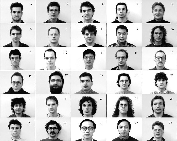
![[*]](http://vismod.www.media.mit.edu/vismod/support/latex2html-98//cross_ref_motif.gif) contains a sample image of
each of the 30 individuals in the database.
contains a sample image of
each of the 30 individuals in the database.
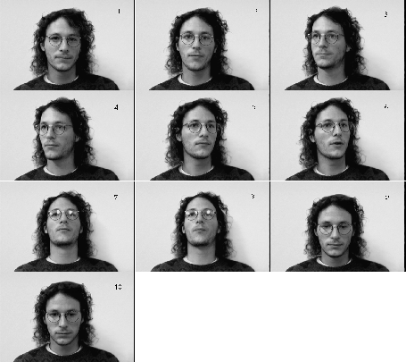
Unlike many other databases which contain only frontal views,
the faces in this database span a variety of depth rotations. The individuals in the
database are presented in 10 different poses. Poses #1 and #2 display the
individual in a frontal pose. Poses #3 and #4 depict the face looking to
the right and poses #5 and #6 depict it looking to the left. Poses #7 and
#8 depict the face looking downwards and poses #9 and #10 depict it looking
upwards. The different views are shown in Figure .
The changes the face undergoes in Figure include large
out-of-plane rotations which cause large nonlinear changes in the 2D images.
Thus, there is a need for an algorithm that can compensate for out-of-plane
rotations, such as the proposed 3D normalization developed in Chapter 4.
For recognition, the algorithm is first trained with 1 sample image for each of the
30 faces. These training images are then stored as KL-encoded keys.
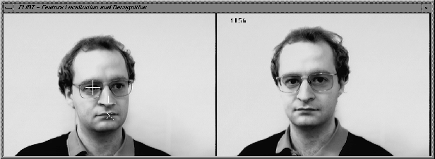
Then each of the 300 images in the Bern database is presented to
the algorithm as a probe image. The system outputs the best match to the probe
from its collection of 30 training images (of the 30 individuals). A sample of
the recognition output is shown in Figure . On the left is
a probe image from the 300-element Achermann database and on the right is the
closest match the system has in its 30 training images.
The number of correct matches and incorrect matches were determined and a
recognition rate of 65.3% was obtained. In other words, of the 300 test
images, the system recognized 196 correctly and 104 incorrectly. Had the
system been purely guessing the identity of the subject, the recognition rate
would be
![]() .
This performance was achieved with only 1
training image per individual in the database. If the number of training
images per individual is increased, superior performance can be expected
[23]. These results are similar to the ones observed by Lawrence
[23] whose recognition algorithm utilizes a self-organizing map
followed by a convolution network. Lawrence achieves 70% recognition accuracy
using only 1 training image per individual. However, his algorithm
requires restricted pose variations. Furthermore, Lawrence tested his algorithm
on the ORL (Olivetti Research Laboratory) database which has more constrained
pose changes than the Achermann database.
.
This performance was achieved with only 1
training image per individual in the database. If the number of training
images per individual is increased, superior performance can be expected
[23]. These results are similar to the ones observed by Lawrence
[23] whose recognition algorithm utilizes a self-organizing map
followed by a convolution network. Lawrence achieves 70% recognition accuracy
using only 1 training image per individual. However, his algorithm
requires restricted pose variations. Furthermore, Lawrence tested his algorithm
on the ORL (Olivetti Research Laboratory) database which has more constrained
pose changes than the Achermann database.
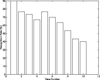
In Figure we plot the recognition rates of the algorithm for
each of the different views (from pose #1 to pose #10) to analyze its
effectiveness to pose variations. As expected, the algorithm fares best with
frontal images (poses #1 and #2). The algorithm recognized the left and
right views (poses #3, #4, #5 and #6) better than the up and down views
(poses #7, #8, #9, #10). It seems that the recognition is more sensitive
to up and down poses. In comparison, most conventional algorithms have
trouble with poses #3 to #10 which are non-frontal.
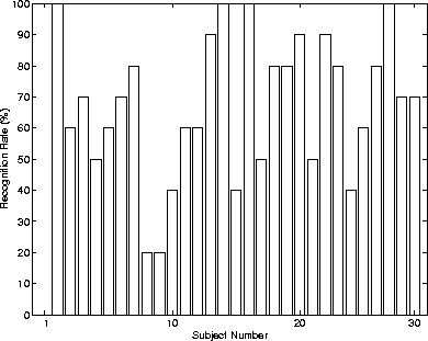
In Figure we plot the effectiveness of the algorithm for each
of the 30 subjects displayed in Figure . Subjects
#1, #8 and #9 were especially difficult to recognize while subjects #2,
#15, #17 and #28 were always recognized. Subjects with particularly
distinct features (such as a beard) were easier to recognize. This is expected
since the algorithm distinguishes faces on the basis of intensity variances.
Thus, large changes in the face induced by beards, etc. cause the most
variance and are easiest to recognize.