Quadratic Bounds

Let us now consider a simple form for the function p, a parabola (or paraboloid in higher dimensions) as in Equation 6.3.

 

$$\begin{array}{ll} p(x) = k - \frac{(x-y)^2}{\sigma} & x \epsilon ... ...y})^T \Sigma^{-1} ({\bf x} - {\bf y}) & {\bf x} \epsilon {\cal R}^n \end{array}$$ (6.3)

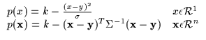
In the above, the parabola contains a maximum which is the scalar value k. It also contains a locus for the maximum which is ${\bf y}$(an element in n-dimensional Euclidean space). Finally, it contains a shape parameter, $\Sigma$ (or $\sigma$ in 1 dimension) which is a symmetric positive semi-definite matrix. There are simpler forms for the bound p (such as a constant or linear function) however the above bound is flexible because it has a single arbitrary maximum, k, at an arbitrary locus, ${\bf y}$. In addition, the maximization of a quadratic bound is straightforward and the maximization of a sum of quadratic bounds involves only linear computation. In addition, unlike variational bounds, the bounding principles used here do not necessarily come from the dual functions (i.e. linear tangents for logarithms, etc.) and are always concave paraboloids which are easy to manipulate and differentiate [53] [51]. Higher order functions and other forms which may be more flexible than quadratics are also usually more difficult to maximize.