Principal Components Analysis

Instead of directly dealing with the redundancies in a large network topology, we will factor out complexity in the input space using a common dimensionality reduction procedure, Principal Components Analysis (PCA) [5]. Consider the a large vector Y(t)composed of the concatenation of all the T vectors that were just observed ${\bf y}(t-1),{\bf y}(t-2),...{\bf y}(t-T)$. Again, as time evolves and we consider the training set as a whole, many large vectors Y (each representing 6 second chunks of interaction) are produced as well as their corresponding subsequent value ${\bf y}(t)$. Therefore the vectors Y contain short term memory of the past and are not merely snapshots of perceptual data at a given time. Thus, many instances of short term memories Y are collected and form a distribution.

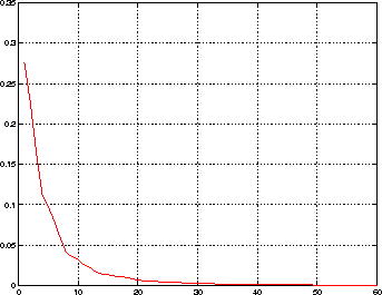
PCA forms a partial Gaussian model of the distribution of Y in a large dimensional space by estimating a mean and covariance. In the ARL system, thousands of these Y vectors are formed by tracking a handful of minutes of interaction between two humans. The PCA analysis then computes the eigenvectors and the eigenvalues of the covariance. The eigenvectors are ranked according to their eigenvalues with higher eigenvalues indicating more energetic dimensions in the data. Figure 4.2 depicts the top few eigenvalues.

  

Figure 4.2: Top 60 Eigenvalues in Y-space

From simple calculations, we see that over 95% of the energy of the Y vectors (i.e. the short term memory) can be represented using only the components of Y that lie in the subspace spanned by the first 40 eigenvectors. Thus, by considering Y in the eigenspace as opposed to in the original feature space, one can approximate it quite well using less than 40 coefficients. In fact, from the sharp decay in eigenvalue energy, it seems that the distribution of Y occupies only a small submanifold of the original 3600 dimensional embedding space. Thus we can effectively reduce the dimensionality of the large input space by almost two orders of magnitude. We shall call the low-dimensional subspace representation of Y(t) the immediate past short term memory of interactions and denote it with ${\bf x}(t)$.

  

Figure 4.3: First Eigenvector of Past Interaction

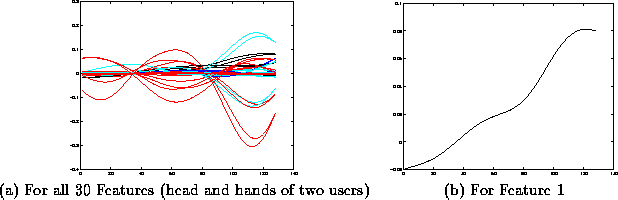
In Figure 4.3 the first mode (the most dominant eigenvector) of the short term memory is rendered as a 6 second evolution of the 30 head and hand parameters of two interacting humans. In addition, it is shown as a 6 second evolution of one of these parameters alone, the x (i.e. horizontal) coordinate of the head of one of the humans. Interestingly, the shape of the eigenvector is not exactly sinusoidal nor is it a wavelet or other typical basis function since it is specialized to the training data. The oscillatory nature of this vector indicates that gestures involved significant periodic motions (waving, nodding, etc.) at a certain frequency. Thus, we can ultimately describe the gestures the participants are engaging in using a linear combination of several such prototypical basis vectors. These basis vectors span the short term memory space containing the Y vectors.