
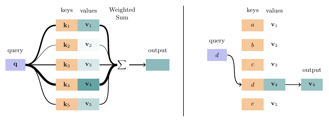
Much of the course so far has been secretly introducing you to the intuitions that led to the most successful neural network architecture so far: the transformer. We know we want an architecture that can make gainful use of lots of parameters. We want residual connections and other optimization-helping tricks, to help train very very deep networks. We want compute efficiency, especially making use of the great parallelization properties of GPUs that we've just learned about. And we have intuitions about building up representations of tokens in a sequence via attention, looking at various places for information useful to the representation at hand.
Here's what we'll do:
As we have come to know and love, let $x_1,\dots,x_n$ be a sequence over finite vocabulary $\mathcal{V}$. As usual, we embed the sequence as $E\x_1,\dots,E\x_n$. Perhaps we encode our position embeddings as we have before (though as we'll see, we may use a different position representation). That is,
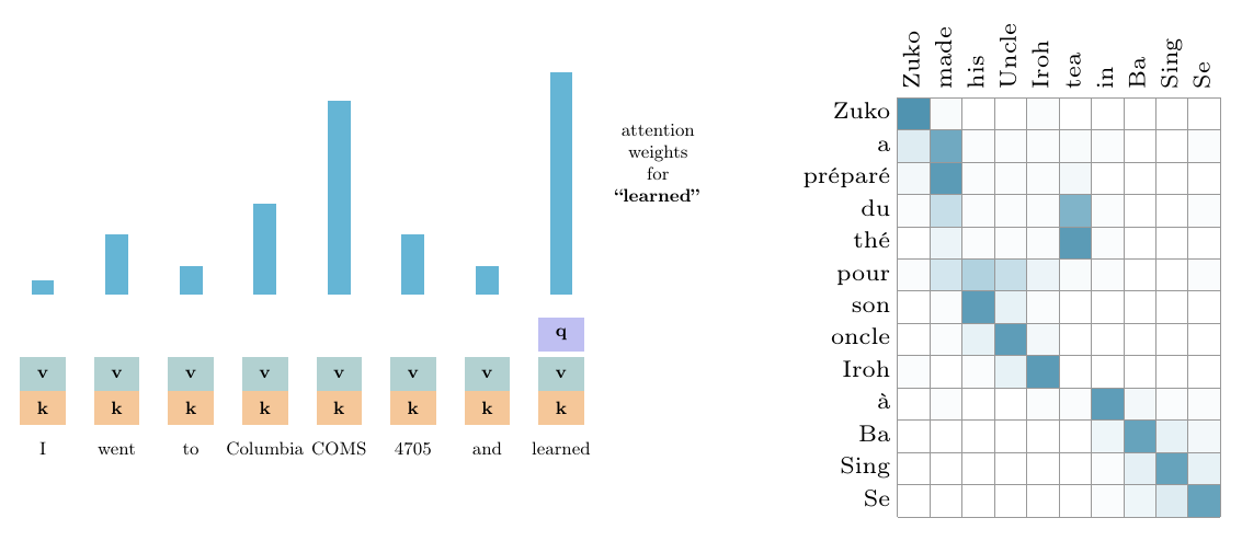
We'll call this sequence $\h_1,\dots,\h_n$. Recall that before, we were computing self-attention, as follows:
So, this uses the vector $\h$ as three things: First, a query: the query is used to search for information in the sequence. Second, a key: the key is like a key in a dictionary, determining what types of queries should access the vector. Finally, a value: the value is what appears in the weighted sum; it's the information that gets passed.
The simplest thing we change first is to allow the keys, queries, and values to be different by linearly transforming each $\h_i$ separately for the three roles. That is, we set
for linear transformations $W_q, W_k, W_v \in \mathbb{R}^{d\times d}$. So now, we compute:
This allows a representation $\h_i$ of a token to be used differently for its different roles. Intuitively, the reason why I might want to look at $\h_i$ (i.e., the key) often times should differ from the content I want from $\h_i$ (i.e., the value.) And then both of these certainly might differ from how $\h_i$ might want to pull in information from previous tokens (the query.)
For a single head, let $\hs\in\mathbb{R}^{n\times d}$ be the matrix with $\h_i^\top$ as its rows.
Because $\q_i = W_q \h_i$, stacking the queries as rows gives $\mathbf{Q} = \hs W_q^\top$ (in code, H @ W_q.T), and likewise for keys and values:
To compute self-attention, we can compute our weights in matrix operations:
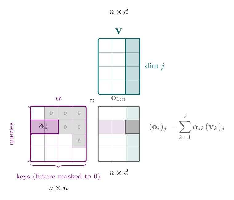
This $\alpha$ is $n\times n$: every query is dotted with every key. In the per-position equations above, the sums ran only up to $i$. Here those limits have to be enforced explicitly, because nothing in the matrix multiply stops index $i$ from looking at $j>i$.
When performing language modeling like we've seen in this course (often called autoregressive modeling), we predict a word given all words so far:
where $f$ is function to map a sequence to a vector in $\mathbb{R}^{|\V|}$.
One crucial aspect of this process is that we can't look at the future when predicting it—otherwise the problem becomes trivial.
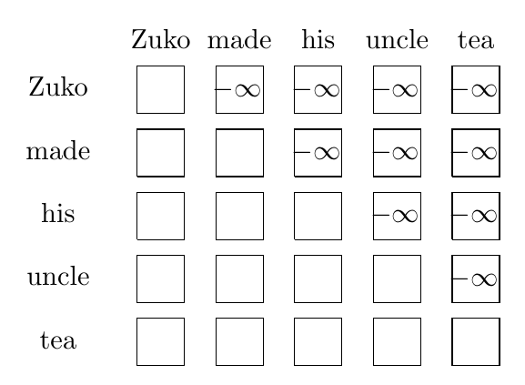
In a Transformer, there's nothing explicit in the self-attention weight $\alpha$ that says not to look at indices $j>i$ when representing token $i$. In practice, we enforce this constraint simply adding a large negative constant to the input to the softmax1
In a diagram, it looks like the figure above. We'll write that additive logit mask as $M$, with $M_{ij}=0$ if $j\le i$ and $M_{ij}=-\infty$ (or a large negative constant) otherwise:
Then the self-attention operation for all positions is:
Here's a pair of diagrams showing the matrix ops, laid out so you can see what gets dotted with what. For the scores, $\mathbf{Q}$ is to the left of $\mathbf{Q}\mathbf{K}^\top$, sharing its $n$ query rows, and $\mathbf{K}^\top$ is above, sharing its $n$ key columns; the inner dimension $d$ meets at the corner and is summed out:
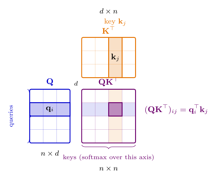
Then for the weighted sum, row $i$ of $\alpha$ (how query $i$ weights every key) dots with column $j$ of $\mathbf{V}$ (dimension $j$ of every value), producing dimension $j$ of the output $\ov_i$. Because of the causal mask, entries $j>i$ of that row are already $0$, so those value rows do not contribute:
Intuitively, a single call of self-attention is best at picking out a single value (on average) from the input value set. It does so softly, by averaging over all of the values, but it requires a balancing game in the key-query dot products in order to carefully average two or more things. In one of your homeworks, you'll work through a bit of this intuition more carefully. What we'll present now, multi-head self-attention, intuitively applies self-attention multiple times at once, each with different key, query, and value transformations of the same input, and then combines the outputs.
For an integer number of heads $H$, we define per-head maps $W_q^{(\ell)}, W_k^{(\ell)}, W_v^{(\ell)} \in\mathbb{R}^{d_h\times d}$ for $\ell$ in $\{1,\dots,H\}$, where $d_h = d/H$ is the head dimensionality. (We'll see why we have the dimensionality reduction to $d_h$ soon.) These are the query, key, and value matrices for each head. Correspondingly, we get queries, keys, and values as in single-head self-attention,
each now in $\mathbb{R}^{d_h}$.
We then perform self-attention with each head:
Note that the output $\ov_i^{(\ell)}$ of each head is in reduced dimension $d_h$. Finally, we define the output of multi-head self-attention as a linear transformation of the concatenation of the head outputs, letting $W_o\in\mathbb{R}^{d\times d}$:
where we concatenate the $H$ head outputs, each in $\mathbb{R}^{d_h}$, into a single vector in $\mathbb{R}^{d}$.
To understand why we have the reduced dimension of each head output, it's instructive to get a bit closer to how multi-head self-attention is implemented in code. In practice, multi-head self-attention is no more expensive than single-head due to the low-rankness of the transformations we apply.
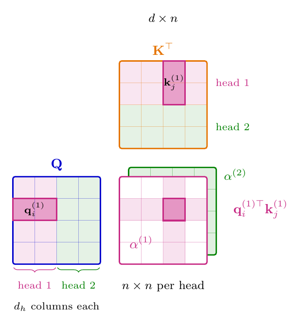
When we perform multi-head self-attention in this matrix form, we pack the per-head maps into a single $W_q \in \mathbb{R}^{d\times d}$ (the vertical concatenation of the $W_q^{(\ell)}$), so $\mathbf{Q}=\hs W_q^\top\in\mathbb{R}^{n\times d}$ as in single-head, and likewise for $\mathbf{K}$ and $\mathbf{V}$. We first reshape $\mathbf{Q}$, $\mathbf{K}$, and $\mathbf{V}$ each into a tensor of shape $\mathbb{R}^{n,H,d_h}$, splitting the model dimensionality into two axes, for the number of heads and the number of dimensions per head. We can then transpose the tensors to $\mathbb{R}^{H, n, d_h}$, which intuitively should look like $H$ sequences of length $n$ and dimensionality $d_h$. This allows us to perform the batched softmax operation in parallel across the heads, using the number of heads kind of like a batch axis (and indeed in practice we'll also have a separate batch axis.) So, the total computation (except the last linear transformation to combine the heads) is the same, just distributed across the (each lower-rank) heads. Here's a diagram like the single-head diagrams, demonstrating how the multi-head operation ends up much like the single-head operation. Each color denotes one head (here $H=2$): after the reshape, head $\ell$'s slice of a query row only ever dots with head $\ell$'s slice of a key column, producing one $n\times n$ attention matrix per head:
Imagine if we were to stack self-attention layers. Would this be sufficient for a replacement for stacked LSTM layers? Intuitively, there's one thing that's missing: the elementwise nonlinearities that we've come to expect in standard deep learning architectures. In fact, if we stack two self-attention layers, we get something that looks a lot like a single self-attention layer:
where $\alpha^*_{ik} = \sum_{j=1}^n\alpha^{(2)}_{ij}\alpha^{(1)}_{jk} = (\alpha^{(2)}\alpha^{(1)})_{ik}$, and $W_v^* = W_v^{(2)}W_v^{(1)}$. So, this is just a linear combination of a linear transformation of the input, much like a single layer of self-attention! Is this good enough?2
In practice, after a layer of self-attention, it's common to apply a feed-forward network independently to each word representation:
where often, $W_1\in\mathbb{R}^{5d\times d}$, and $W_2\in\mathbb{R}^{d\times 5d}$. That is, the hidden dimension of the feed-forward network is substantially larger than the hidden dimension of the network, $d$—this is done because this matrix multiply is an efficiently parallelizable operation, so it's an efficient place to put a lot of computation and parameters.
One important learning aid in Transformers is layer normalization (Ba et al., 2016). The intuition of layer norm is to reduce uninformative variation in the activations at a layer, providing a more stable input to the next layer. Further work shows that this may be most useful not in normalizing the forward pass, but actually in improving gradients in the backward pass (Xu et al., 2019).
To do this, layer norm (1) computes statistics across the activations at a layer to estimate the mean and variance of the activations, and (2) normalizes the activations with respect to those estimates, while (3) optionally learning (as parameters) an elementwise additive bias and multiplicative gain by which to sort of de-normalize the activations in a predictable way. The third part seems not to be crucial, and may even be harmful (Xu et al., 2019), so we omit it in our presentation.
One question to ask when understanding how layer norm affects a network is, “computing statistics over what?” That is, what constitutes a layer? In Transformers, the answer is always that statistics computed independently for a single index into the sequence length (and a single example in the batch) and shared across the $d$ hidden dimensions. Put another way, the statistics for the token at index $i$ won't affect the token at index $j\not=i$.
So, we compute the statistics for a single index $i\in\{1,\dots,n\}$ as
where (as a reminder), $\hat{\mu}_i$ and $\hat{\sigma}_i$ are scalars, and we compute the layer norm as
where we've broadcasted the $\hat{\mu}_i$ and $\hat{\sigma}_i$ across the $d$ dimensions of $\h_i$. Layer normalization is a great tool to have in your deep learning toolbox more generally.
Residual connections simply add the input of a layer to the output of that layer:
the intuition being that (1) the gradient flow of the identity function is great (the local gradient is 1 everywhere!) so the connection allows for learning much deeper networks, and (2) it is easier to learn the difference of a function from the identity function than it is to learn the function from scratch. As simple as these seem, they're massively useful in deep learning, not just in Transformers!
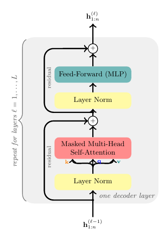
In the Transformer diagrams you'll see, including the decoder-layer figure below, the application of layer normalization and residual connection are often combined in a single visual block labeled Add & Norm. Such a layer might look like:
where $f$ is either a feed-forward operation or a self-attention operation, (this is known as pre-normalization), or like:
which is known as post-normalization. It turns out that the gradients of pre-normalization are much better at initialization, leading to much faster training (Xiong et al., 2020).
Another trick introduced in Vaswani et al. (2017) they dub scaled dot product attention. The dot product part comes from the fact that we're computing dot products $\q_i^\top \K_j$. The intuition of scaling is that, when the dimensionality $d_h$ of the vectors we're dotting grows large, the standard deviation of the dot product of even random vectors (e.g., at initialization) grows roughly as $\sqrt{d_h}$. So, we normalize the dot products by $\sqrt{d_h}$ to stop this scaling:
Putting the pieces together, the figure below shows one decoder layer: layer norm, then masked multi-head self-attention, then a residual connection; then layer norm, then the MLP, then another residual connection. A Transformer decoder is a stack of $L$ of these layers (each with its own parameters), with the output $\h^{(\ell)}_{1:n}$ of layer $\ell$ serving as the input to layer $\ell+1$.
Often in practice, we think of two different ways of running a transformer on a GPU: sampling and prefill. Sampling means generating tokens one at a time (according to our usual autoregressive process) and prefill means building the representations for a whole sequence of tokens at once. The math is the same in both—the equations we've written don't change. However, the information we have access to differs depending on whether we're sampling (by our intention, we don't know the future tokens yet) or prefilling (we know the whole sequence and want to run the model all at once.) As a concrete motivation, you'll notice that input tokens are much cheaper than output tokens in common LLM API pricing schemes (like those of OpenAI or Anthropic.) This motivates why.
When performing prefill (say, to compute the log-likelihood of a known sequence,) we get to run our batched attention operation basically as written here. A few very large matrix multiplies. However, when sampling, the lack of knowledge of future tokens means that whenever a new token is generated, we're constructing the activations just for that one token at each layer, and computing attention computations for all previous tokens. We thus need to have cached the activations for previous tokens, in order to go back and reference them when computing attention. In practice, we cache key and value vectors, calling it a KV-cache. At each layer of the transformer, we thus apply our residual connections and MLPs (those only depend on the current timestep activation) and then use our KV-cache to compute our attention scores over the history. The figure below shows the sampling-time picture: keys and values for the prefix live in the KV-cache, the current token's key $\K_t$ and value $\va_t$ are appended to it, and the current query $\q_t$ is dotted against every key in the cache (including its own, since the mask allows $j\le t$).
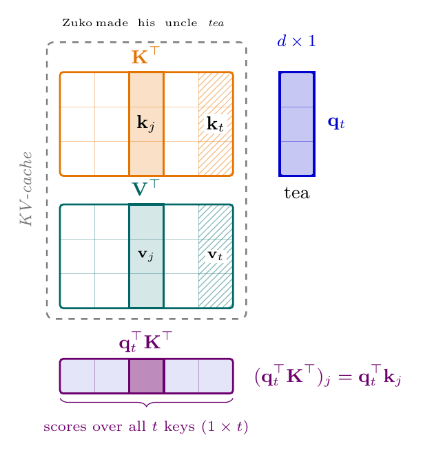
At sampling time, the KV-cache grows over time as we sample. Our sampled sequences may become very long (thousands to millions of tokens,) meaning the GPU memory cost of keeping the KV cache around becomes prohibitive. There are a ton of systems-level ideas for computing (or approximating) this efficiently while limiting memory usage, but here we'll talk about two popular model architecture tweaks that reduce the total necessary memory for the KV-cache.
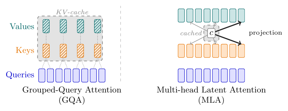
The first is grouped query attention (Ainslie et al., 2023), which keeps the number of queries as the number of heads $H$, but computes fewer keys and values, assigning multiple queries to each key/value pair. Intuitively, this approximates full multi-head attention by allowing for a lot of reasons to look up information (queries) but reduces the storage (and thus possible independent types of information.) The figure below (left) shows the grouping: pairs of query heads share a key and value, so the KV-cache stores $G$ heads instead of $H$.
The second is multi-head latent attention (MLA) (DeepSeek-AI, 2024). Instead of explicitly producing and storing keys and values, MLA computes and stores a single memory vector $c = W^{\text{DKV}}h$ for an activation $h$. The dimensionality $d_{\text{dkv}}$ should be much less than the total dimensionalities of keys and values, (heads times dimensions per head times two, $2hd_h$.) At inference time, the memory vector is linearly transformed back up to $2hd_h$ (and reshaped) to be used as keys and values. Cool! The figure below (right) shows this: keys and values are not cached; only the compressed latent is.
tbd
tbd
tbd
float16 encoding is used instead, like $-10^4$. Using infinity can lead to NaNs and it's sort of undefined how each library should treat infinite inputs, so we tend to avoid using it. And because of finite precision, a large enough negative constant will still set the attention weight to exactly zero. ↩