
In this note, we discuss TPUs, GPUs, what it means for neural network architectures to be parallelizable across these accelerators, and implications for neural network design. The goal is not to make you adept at writing CUDA code—the code that directly specifies GPU behavior—but to teach you enough about the structure of GPUs (and a bit about TPUs) to help you reason through the design and implementation of your neural networks.
A good neural network architecture learns flexibly and efficiently from data. By flexibly, we mean that the network is expressive, as we’ve discussed before in this course. To recall, a network architecture is expressive when it can express complex functions and learn such functions from data.
By learning efficiently, one of three things is usually meant. One is data efficiency, wherein one measures performance of a network in the architecture as a function of the number of training samples shown, desiring as high performance as possible for any sample budget. Another is time efficiency, wherein one measures performance of a network in the architecture as a function of how long it takes, in seconds, to complete. The third is flop efficiency, measuring how many floating-point operations are needed to compute the training. Note the distinction between time efficiency and flop efficiency—if I have a ton of machines, I might not care about low flop-efficiency as long as my algorithm allows me to use all my machines to compute the function faster in terms of seconds.
Which one seems more important? In some sense, counting the number of operations feels like the more standardizable unit—wall clock time must depend on all kinds of things like what hardware is being used, whether other programs are running, or how fast one’s disk I/O is.
However, modern LLM development has taught us that the first-order term in the approximation of neural network quality is how much computation you spend on showing reasonably high-quality data to a model. To grossly oversimplify, model quality is something like:
Of course, this isn't real math, and one should at least break down good data into terms about data quality and quantity, and what kind of compute... But scaling compute just helps. The amount of computation is roughly:
This means we want to define architectures that maximize the amount of computation we can achieve for a fixed amount of wall-clock time. This in turn means defining architectures that suit the computing hardware we have.
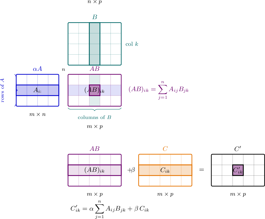
Consider matrices $A\in\mathbb{R}^{m\times n}$ $B\in\mathbb{R}^{n\times p}$, and $C\in\mathbb{R}^{m\times p}$. Also consider scalars $\alpha,\beta\in\mathbb{R}$. We've seen matrix multiplication $AB$, and we've seen addition of matrices (or vectors) $AB+C$. A general matrix multiplication is an operation of the form
where $C$ is an existing matrix that is overwritten by the operation. (We haven't talked about things like memory usage yet in the course, but this is where it starts, so keep in mind that it matters that we already had memory around storing $C$; we're not adding in some other unrelated matrix $D$.) From this operation we can recover, e.g., matrix multiplication by setting $\beta=0,\alpha=1$:
Note that the technical content in this section so far is basically drawn from NVIDIA's great matrix multiplication user guide. This will be true of much of the content in this article, though I'll be adding a few bits here and there, and removing some of the details I don't think are critical for this course.
We've seen plenty of matrix multiplies in the course. Here are a few, with some example dimensionalities. First off, the matrix multiply just before the softmax in our language model
We usually have thought of this as a matrix-vector multiply, $E\in \mathbb{R}^{|\mathcal{V}|\times d}$, and $h\in\mathbb{R}^d$. But as you see in assignment 1, we often compute these quantities over, e.g., a whole sequence, so our $h\in\mathbb{R}^{d\times T}$ is the matrix of all $h$ vectors for a whole sequence of $T$ words. Now we can see we have a GEMM with shapes $(|\mathcal{V}|, d)$, $(d, T)$, and $(|\mathcal{V}|, T)$, with the pre-existing $C=0$.
We've also seen the selection of a word embedding by multiplying by a one-hot vector $w$:
where $w=[0;\cdots;1;0;\cdots]\in\mathbb{R}^{|\mathcal{V}|}$ selects a particular vector in $\mathbb{R}^{d}$ from $E$. This can be re-written as an index lookup from $E$.
One operation that is a matrix operation but is not a matrix multiply is the averaging in our averaging language model:
GPUs (Graphics Processing Units) and TPUs (Tensor Processing Units) are computing hardware specialized to perform a large number of independent operations in parallel. This specialized functionality is in contrast to CPUs, which excel at serial operations—operations performed one after another, thus allowing future operations to depend on the results of earlier operations.
Serial computation is more flexible by allowing these dependencies. However, parallel computation allows us to scale the number of operations performed at once, since no operation has to wait for another.
If you have the time, I recommend reading this great article on GPU performance released by NVIDIA. A lot of what I'll write in this subsection is drawn from that. I'll also draw from the related matrix multiply users guide here.
A GPU is an accelerator with its own memory and computing cores, separate from the CPU of the machine that the GPU resides on. Our goal here is to discuss enough of the data and computation model of the GPU to write reasonably performant neural network programs. However, there's a lot of room for much more efficiency by digging into details that we won't cover in this course!
Let's start by looking at the figure below. At the left, we see the machine RAM, which I've labelled as 512GB. Even before this, we have the hard disk storage of the machine (which might be terabytes (1000s of GB) large.) Let's say we have a matrix in $A\in \mathbb{R}^{512\times 512}$ and we want to compute $A^2$. First off, let's say we're representing the values of $A$ in 32-bit floats. That means each of the $512*512$ floating point numbers we need each takes $4$ bytes, so we have a total of $512*512*4=2^{20}$ bytes. If $A$ resides on our hard disk, we first read it to the machine RAM (slow). From the machine's RAM we move a matrix to the GPU RAM, which tends to be much smaller (For example, a top-of-the line B200 GPU has 192GB; a T4 has 16GB.) To compute $A^2$, we further move parts of $A$ in chunks to the caches and registers of the streaming multiprocessors. We won't get into the streaming model here, but consider that each dot product in $A^2$ does not depend on any other; they can be computed parallel. The result of computing $A^2$ is written back to GPU VRAM (and must separately be explicitly moved back to the CPU RAM if you want it there.)
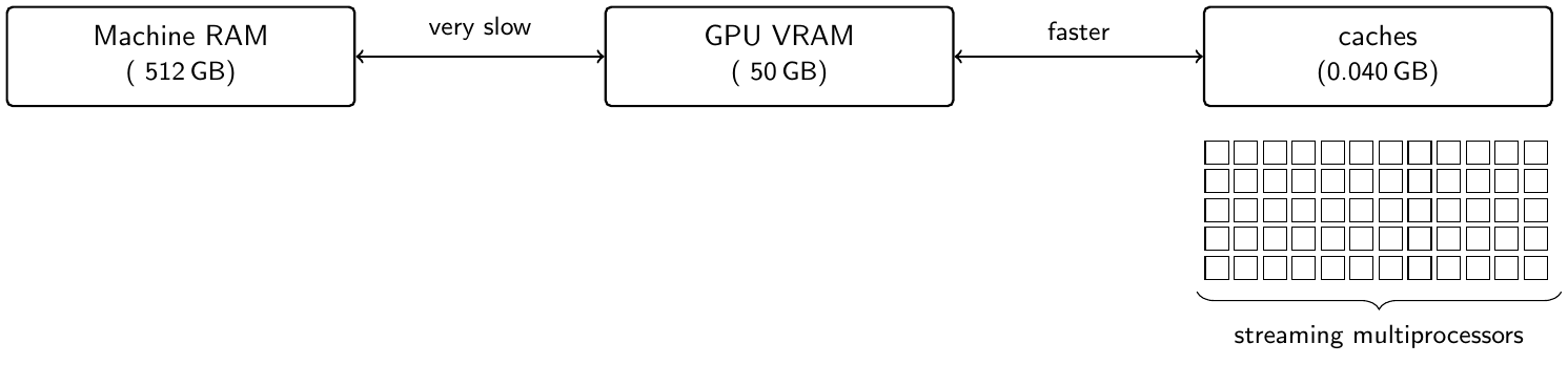
So, there are two things we do when computing our operation: we move around bytes (memory access) and we actually perform math. Let's call $T_{\text{math}}$ the time we spend doing math and $T_{\text{mem}}$ the time we spend accessing memory. Assuming we can overlap these two (again, see the NVIDIA blog post) our time for our program is
If $T_\text{mem}$ is greater than $T_{\text{math}}$, our program is memory-bound. If instead $T_\text{math}>T_{\text{mem}}$, the program is math-bound. As we'll see, we're often memory-bound.
To approximate $T_\text{math}$ and $T_{\text{mem}}$, we can use the following rough calculation. Let $C_\text{mem}$ be the number of bytes we access for our computation. Let $C_{\text{math}}$ be the number of floating-point operations (e.g., scalar multiplications.) The ratio of these two is called the arithmetic intensity:
If we let $B_{\text{math}}$ be the math bandwidth (or, speed at which we compute mathematical operations) and $B_{\text{mem}}$ Be our memory bandwidth (speed at which we access/move memory)
A processor's operations-to-byte ratio is then:
Our time taken for math operations and memory access respectively are:
and our program is memory-bound if:
Matrices of $m \times k$ and $k \times n$ leads to $m \times n$ matrix. Uses $mnk$ FLOPs. Memory accesses: $mk$ + $kn$ + $mn$ (for output.) Arithmetic intensity is:
Here's an example using small matrices. Let's use $m=10$, $n=20$, and $k=30$:
For $C_\text{math}$, we have:
And for $C_\text{mem}$:
so an arithmetic intensity of:
Now, let's use $m=1000$, $n=2000$, and $k=3000$. For $C_\text{math}$, we have
and for $C_\text{mem}$:
for an arithmetic intensity of: