
The main innovation that has moved methods in natural language processing from largely not working to largely working is pretraining. At a high level, this idea returns exactly to the start of the course. Pretraining means trying to learn from a huge amount of text (and usually now also images, video, audio, etc. But we'll focus on text.) All of the topics we've covered so far — expressivity of neural networks, optimization, tokenization, and parallelizable architectures — are to some extent in service of better pretraining.
The method we introduced in lecture 1 is similar to word2vec (Mikolov et al., 2013), and we saw that our simple word prediction algorithm led to very interesting learned structure. By scaling up the expressivity of the architecture and the scale, interesting things keep happening!
What predictive problem are we going to be training our network on? You guessed it, language modeling. Recall that we have some learnable parameters $\theta$ in our distribution $p_\theta$, we have a data distribution $\mathcal{D}$, and we're going to optimize:
But at this point let's get a bit more specific. This math suggests that we're optimizing specifically over entire documents. In practice, something slightly messier happens.
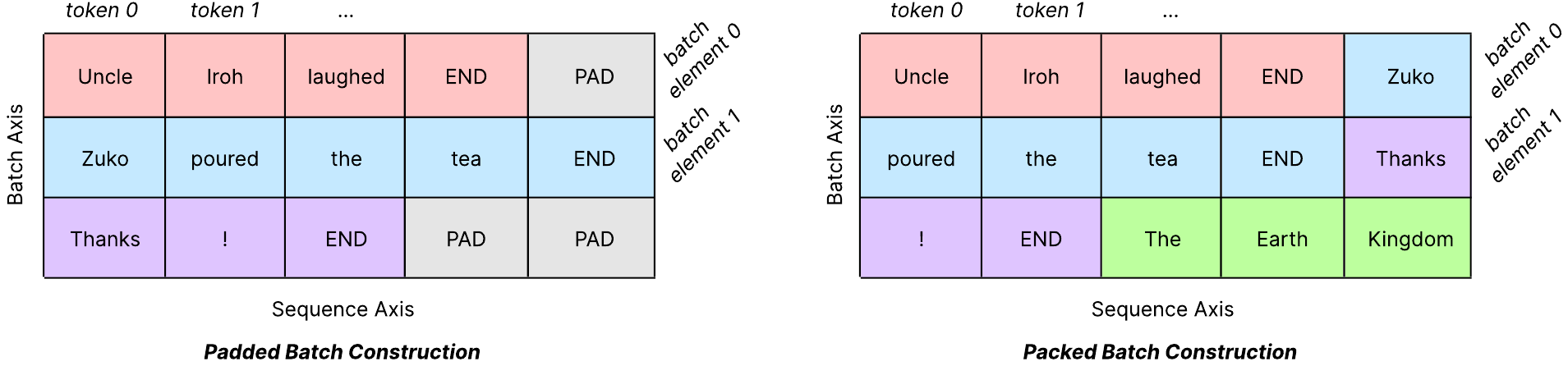
Let's say I have a batch size $B$ and a maximum sequence length $n$. I've probably set $B$ and $n$ such that I have as long sequences as I can, and as large a batch as I can, such that it'll fit on my GPU cluster. So, that's $Bn$ tokens I can potentially learn from. However, if I try to optimize the math above, suggesting that I optimize for the likelihood of whole documents, this means I need to filter out documents longer than $n$ tokens. Furthermore, any documents shorter than $n$ tokens I need to pad with useless blanks that won't be trained on, in order to fill out the batch. That's wasted compute!
Instead, batches are packed with tokens. That is, we string together a bunch of documents and just pick the first $Bn$ tokens, even if they cross document boundaries. If they do cross document boundaries, we include a document separator token.
We then optimize a similar-looking objective over this new distribution over tokens, call it $\tilde{\mathcal{D}}$.
This is a bit of a technical detail — much of the time we're still optimizing document likelihoods, but not always due to the packing (figure above), but I think it helps build intuition — we're looking for useful token sequences to learn from, and a lot, as fast as possible.
First, consider the size of datasets that are used in practice for pretraining models such as the GPT series of models. In June of 2018, the initial idea of a generative pre-trained transformer (GPT) was introduced by Alec Radford and others at OpenAI (Radford et al., 2018). The GPT-1 model has 117 million learnable parameters, and was trained on the BooksCorpus, containing roughly 985 million words or 1.3 billion tokens. With this size and training, the model was already able to do interesting things by primarily learning to predict the next token. Later, in 2019, Radford and others released GPT-2 (Radford et al., 2019) which has 1.5 billion learnable parameters and was pretrained on a large corpus of web text containing 8 million documents and roughly 21 billion tokens. In 2020, OpenAI then announced GPT-3 (Brown et al., 2020) with 175 billion parameters trained on an estimate $\sim$500 billion tokens of CommonCrawl data. Finally, GPT-4 (OpenAI, 2024) and GPT-5 were announced in March, 2023 and August 2025 respectively, but we don't really know details about the size of the model or training corpus.
Some other common, recent models and their associated parameter counts are listed in the table below. Many current leading models have hundreds of billions of tokens and are trained on tens of trillions of tokens.
| Model | Provider | Model Size (# Parameters) | Corpus Size (# Tokens) |
|---|---|---|---|
| OLMo-2 | AllenAI | 7–13 billion | 5 trillion |
| Gemma 3 | 270 million – 27 billion | 6–12 trillion | |
| DeepSeek-V3 | DeepSeek AI | 685 billion | 14.8 trillion |
| Llama 3 | Meta | 7–405 billion | 15 trillion |
| Qwen3 | Alibaba | 235 billion – 1 trillion | 36 trillion |
Common large language models with their size and number of training tokens. Ranges of model sizes indicate that multiple models of different sizes were part of the same named release (e.g., Gemma-3-8B and Gemma-3-27B).
Take a look at the FineWeb examples table below. Here are two ``real'' pretraining documents from FineWeb (Penedo et al., 2024).
What token sequences should we learn from? Sometimes we approximate the training distribution of language models as the whole internet, but this is wrong for various reasons. Still, it's a useful intuition, and a large part of pretraining datasets is often Common Crawl dumps, which are large public crawls of the internet. But cleaning, filtering, formatting the text in raw crawls is critical.
Here are some types of filtering or processing found in the FineWeb dataset (Penedo et al., 2024):
To put some of these pre-processing steps in perspective, consider the texts removed by each of several steps in the figure below. Beginning with a pool of CommonCrawl texts, DataCompLM removes nearly 99% of the original documents to curate a corpus for pretraining, and the final corpus still contains roughly 2–3 trillion tokens. While most documents are removed by filters similar to those listed above (e.g., language filters, deduplication), the final step, model-based filtering, primarily concerns selecting the kinds of documents we think would be best for pretraining.
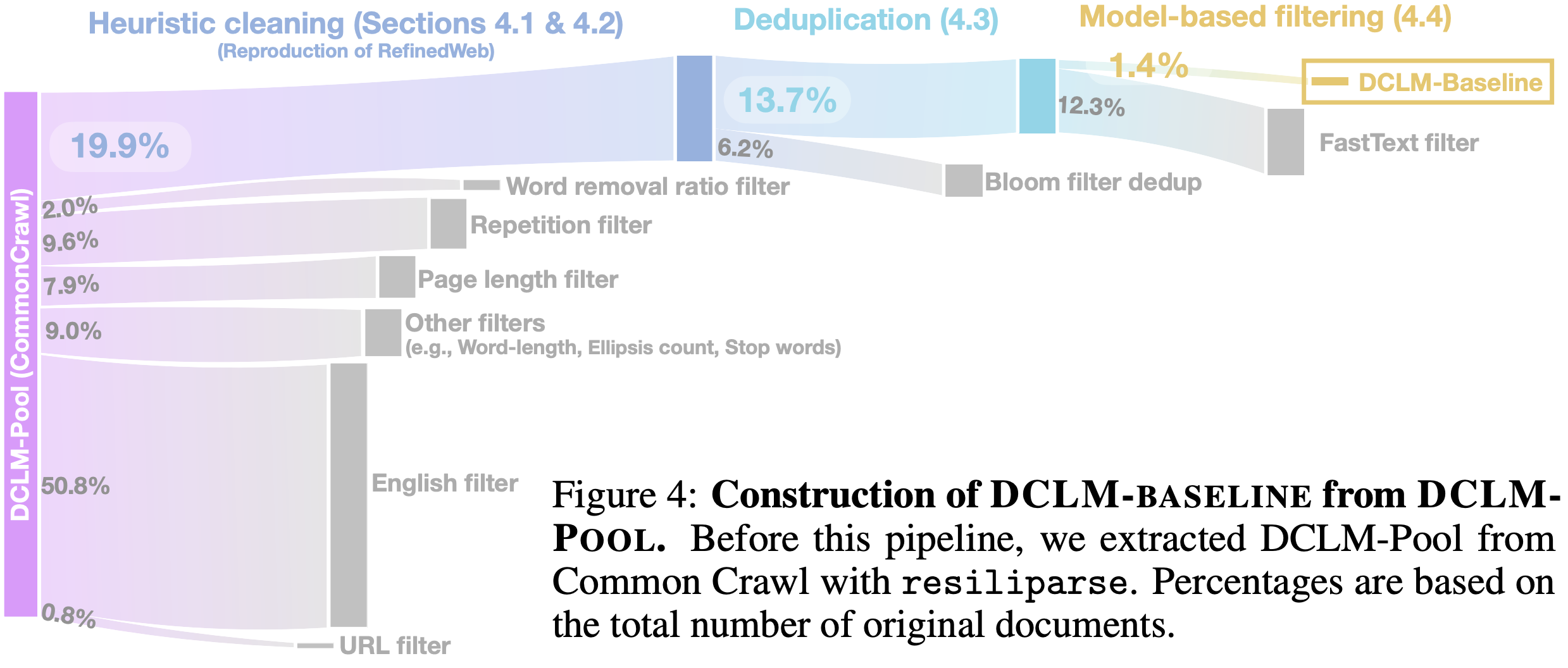
It's very expensive to test hypotheses about what kind of web data is best for pretraining. Vaguely, some notion of quality is usually used — Wikipedia is high quality, random web pages might be low-quality. One nice concrete intuition is as follows, however.
In DataCompLM, they trained models to score each web document with how alike it is to a combination of Reddit Explain-Like-I'm-Five data and a synthetically generated question-and-long-response chatbot dataset called OpenHermes2.5 (Teknium, 2024). That is, when filtering down from a raw web dump, documents are kept when the model predicts that they're more like these sources. And this worked very well!
| FineWeb Examples |
|---|
|
Previous abstract Next abstract Session 40 - The Interstellar Medium. Display session, Tuesday, June 09 Gamma Ray Burst (GRB) explosions can make kpc-size shells and holes in the interstellar media (ISM) of spiral galaxies if much of the energy heats the local gas to above $10^7$ K. Disk blowout is probably the major cause for energy loss in this case, but the momentum acquired during the pressurized expansion phase can be large enough that the bubble still snowplows to a kpc diameter. This differs from the standard model for the origin of such shells by multiple supernovae, which may have problems with radiative cooling, evaporative losses, and disk blow-out. Evidence for giant shells with energies of $\sim10^{53}$ ergs are summarized. Some contain no obvious central star clusters and may be GRB remnants, although sufficiently old clusters would be hard to detect. The expected frequency of GRBs in normal galaxies can account for the number of such shells. Program listing for Tuesday |
|
Wikipedia sobre física de partículas Rapidinho. Me falaram que a definição de física de partículas da Wikipedia era muito ruim. E de fato, era assim: Particle physics is a branch of physics that studies the elementary particle|elementary subatomic constituents of matter and radiation, and their interactions. The field is also called high energy physics, because many elementary particles do not occur under ambient conditions on Earth. They can only be created artificially during high energy collisions with other particles in particle accelerators. Particle physics has evolved out of its parent field of nuclear physics and is typically still taught in close association with it. Scientific research in this area has produced a long list of particles. Mas hein? Partículas que só podem ser criadas em aceleradores? Física de partículas é ensinada junto com física nuclear? A pesquisa produz partículas (essa é ótima!)? Em que mundo essa pessoa vive? Reescrevi: Particle Physics is a branch of physics that studies the existence and interactions of particles, which are the constituents of what is usually referred as matter or radiation. In our current understanding, particles are excitations of quantum fields and interact following their dynamics. Most of the interest in this area is in fundamental fields, those that cannot be described as a bound state of other fields. The set of fundamental fields and their dynamics are summarized in a model called the Standard Model and, therefore, Particle Physics is largely the study of the Standard Model particle content and its possible extensions. Eu acho que ficou bem melhor. Vamos ver em quanto tempo algum editor esquentado da Wikipedia vai demorar para reverter. Atualmente está um saco participar da Wikipedia por causa dessas pessoas. |
Some example documents from FineWeb. Note that they're still pretty messy.
As mentioned, if Wikipedia is primarily high quality, why can't we just train a model only on Wikipedia texts? All of English Wikipedia contains roughly 5–7 billion tokens1. In contrast, however, the original GPT-2 model training used more than 21 billion tokens of text. Therefore, we need a method to estimate the quality of documents outside of known sources like Wikipedia.
While some other approaches exist2, the approach taken in DataCompLM to score the quality of documents based on known sources is similar to many of the model-based filtering approaches often used to filter pretraining corpora. Assume you have a pool of documents, $\mathcal{D} = \{D_1, D_2, ..., D_N\}$ that you may want to use to pretrain your model where each document is a string over a finite vocabulary, $D_i = w_1,...,w_T$. Given that quality is difficult to define precisely, it is unlikely we will come up with a good approach to label each document as definitively ``bad'' or ``good''. So, the aim of model-based quality filtering is to instead sort this set of documents by there quality.
Taking sources of documents that we assume are high quality (i.e., Wikipedia), we can train a classifier defined by $f(D) \mapsto c$, where the output, $c$, is a value $[0,1]$ represents the probability that $D$ could be from our high quality sources. If Wikipedia is our high quality source for example, we train this classifier to prioritize (i.e., give a high score to) documents that look like or contain Wikipedia text and de-prioritize (i.e. give a low score to) documents that don't look like Wikipedia text. We can then label each document with this classifier, sort our training pool by the associated score, and take the highest scoring documents as our pretraining data.
To train these model-based filters, we can use much of what we have learned in the course so far. Instead of predicting the next token, however, we instead want to perform binary classification that will output a single quality score. If we remove the final linear layer and softmax of a transformer, we instead get a vector corresponding to the last token of the input, $h = \text{Transformer}_{\theta}(D)$ where $h \in \mathbb{R}^d$ and $\theta$ represents all learnable parameters of the transformer. Intuitively, this $h$ is the best representation of the document we can extract from the model given it incorporates some information about all prior tokens in the sequence through all layers of the model.
Using this representation from the model, we define a new model as follows:
where $g$ is a small set of learnable parameters in $\mathbb{R}^d$ defining the classifier. Then, we can define a loss function for this classifier and use gradient descent to train all parameters. Formally, we could try to optimize the score given to documents from Wikipedia (or another high quality source):
This formulation, however, can be trivially optimized by always predicting $f(D) = 1$ because it lacks negative examples. So, we modify our training by assuming that generally, any other documents that we sample besides Wikipedia documents are, on average, worse than Wikipedia. While this may result in a poor classifier if we relied on binary labels, remember that we only need to sort our pool of training data by their similarity to Wikipedia rather than discretely classify documents as high or low quality. So, we instead optimize:
Part of the promise of pretraining is that it's been shown to work (and thus is to some extent predicted to work) across many orders of magnitude. This is especially important because of the immense costs of scaling to each additional order of magnitude. See the figure below, in which scaling the amount of computation, the amount of data, and the number of parameters leads to a decay in loss that scales linearly with the logarithm of the increase in cost. While sometimes stated as natural laws, I think of them as useful estimates.
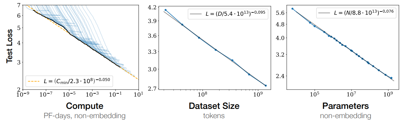
Given this predictable relationship, we can attempt to determine the ``optimal'' tradeoff between scaling the number of parameters and the number of tokens a model is trained on. Specifically, work has investigated how we can empirically determine this tradeoff. To do so, they fit a function that predicts the loss a transformer model will achieve at the end of pretraining (Hoffmann et al., 2022), which is of the form
In this function, $\hat{L}(N, D)$ represents the predicted loss (similar to what we have seen earlier in the course) based on the number of parameters ($N$) and the number of training tokens ($D$). As there is inherit uncertainty in predicting the next word of real language, the first term, $E$, represents the minimum achievable or ideal loss of the model. The second term, $\frac{A}{N^\alpha}$, represents the added loss due to having too few parameters, while the third term, $\frac{B}{D^\beta}$, represents the added loss due to not training on enough data. Among the constants in this function, $\alpha$ and $\beta$ represent the rates of improvement gained when scaling the number of parameters and the number of training tokens respectively. Therefore, knowing these values of these rates provides general guidelines for how to scale the number of parameters and training tokens relative to each other in order to achieve the optimal loss.
After fitting this function to real model training runs and losses, the authors estimated that the relevant scalar values are roughly $\alpha \approx \beta \approx 0.5$. Because $\alpha$ and $\beta$ are found to be similar, this means that optimally, the number of parameters and the number of training tokens should be scaled similarly to each other.
This optimal tradeoff, however, is generally not followed in practice; while this function gives insights into how to optimally use a computational budget to minimize the resulting training loss, it does not take into account the costs of model inference. Smaller models are less costly to run, so model developers generally choose instead to tradeoff more time spent pretraining and more tokens to keep the costs of model inference to users low.
Through pretraining on a broad range of text, we've come to a probability distribution $p_{\theta_p}$. We might not want to sample from this distribution, though! However, we also have the learned parameters $\theta_p$ themselves, of a neural network. These parameters can serve as the initialization of an optimization problem for more specific task. This is finetuning. It is a fascinating empirical fact of neural networks that the pretrained parameters $\theta_p$ are an excellent starting point.
Consider a dataset $\mathcal{D}= \{(x_i, y_i)\}_{i=1}^{m}$ of examples, where each $x_i\in\mathcal{V}^*$, and $y_i\in\mathcal{V}^*$. We want a probability distribution that generates outputs like the $y$ when given inputs like the $x$. We have $\theta_p$ to start with. We're going to take minibatches from $\mathcal{D}$, start with $\theta_0=\theta_p$, and then run stochastic gradient descent:
So, we're just optimizing over the parameters of our network the same loss function had we started from a random initialization instead of our pretrained $\theta_p$. But we're hoping that starting from where we do will lead to good things. And in practice it does! But one should ask, why? When we write out an optimization problem:
if we do a great job of computing that minimum, it shouldn't matter so much where we start. In general, non-convex optimization is hard, though, so maybe starting from $\theta_p$ helps us achieve a lower minimum loss. Unfortunately, this isn't really true either. Even for relatively large datasets $\mathcal{D}$, for the large neural networks that we use, we can tend to achieve roughly minimum (e.g., 0) loss via gradient descent even without pretrained initialization. So, if pretraining does not necessarily make optimization better, why would we want to start from $\theta_p$?
At a high level, the success of finetuning is due to the parameters of the network not straying “too far” from the pretrained parameters. The pretrained parameters $\theta_p$ lead to building all sorts of interesting representations, similarities between words and phrases with similar meanings, subskills relating to understanding language. When finetuning, we leverage these learned representations, and just “tweak” them a bit such that the output distribution is what we'd like. Let's use an example to demonstrate this.
Consider two models: $\theta_0$, which has randomly initialized parameters, and $\theta_p$, our pretrained model. We train both of them on the dataset $\mathcal{D}= \{(x_i, y_i)\}_{i=1}^{m}$, where $x_i$ is a question about a university's location and $y_i$ is the corresponding answer. For example, one training pair could be (Q: Where is the University of Pennsylvania?, A: Philadelphia). Now, if we select an example from the held-out set — say, Q: Where is Pennsylvania State University? — and ask both models to predict its location, what answers could we get? The randomly initialized model $\theta_0$ might output a biased answer such as “Philadelphia”, since “Pennsylvania” and “Philadelphia” could have close embedding space. In contrast, the pretrained model $\theta_p$, having likely seen information about Pennsylvania State University during pretraining on large-scale web data, would be more likely to output the correct answer, State College. Therefore, by starting from $\theta_p$, we encourage the model not to stray “too far” from its pretrained parameters. In other words, finetuning mainly adjusts our desired model behavior, such as its format of response, instead of changing the actual information it has already learned.
The intuition of not straying “too far” from the pretrained parameters is nice because we can try to define what “too far” means, and develop our intuitions. One natural idea is $L_2$ distance — simply, in a natural vector space metric, how much have we moved due to gradient descent?
Is this the right notion of distance in our finetuning? One way of exploring this is to run our optimization procedure with an explicit penalty on $L_2$ distance, as follows:
where $\beta$ is a hyperparameter deciding the relative importance of not moving too far in weight space. This is called an $L_2$ penalty, and it's a reasonable strategy, but in practice isn't used too much. Intuitively, this penalizes every single parameter equally for how much it strays from its initial position, and maybe some parameters should move a lot, while others shouldn't move much at all.
Another interesting space to measure “too far” in is distributional space. Instead of penalizing the deviation of the parameters themselves, maybe we want to make sure our learned distribution $p_\theta$ isn't too different from the pretrained distribution $p_{\theta_p}$. One way to do this is to decide a distribution over text, say $\mathcal{T}$ and then penalize the KL-divergence of the token-level distributions of each model on the prefixes defined by that text:
Recall that $p_{\theta_p}(\cdot \mid x_{\lt t}) $ is a $|\mathcal{V}|$-sized categorical distribution over tokens $x_t$ given prefix $x_{\lt t}$, and the KL-divergence of one such conditional distribution is
where $p_{\theta_p}(w \mid x_{\lt t})$ is the weight of token $w$ according to $\theta_p$, and $\frac{p_{\theta_p}(w \mid x_{\lt t})}{p_{\theta}(w \mid x_{\lt t})}$ shows how different $p_{\theta_p}$ and $p_{\theta}$ are for that token prediction. So, if the pretrained distribution places a lot of probability on a word in a given prefix and our finetuned distribution does not, the parameters are penalized and pushed towards placing more probability on that word. Is this the right intuition for not straying too far from the pretrained parameters? Sort of, sometimes. Intuitively, sometimes we want to change the distribution quite a bit — say we pretrained mostly on English text, but we want to finetune on translation to Tamil. It turns out that the English pretraining is still quite useful for this task, despite the pretrained distribution being quite different from the one we'd like. Therefore, we can add this KL penalty as an extra objective, which is a common tool. So now, the objective becomes:
Together, this objective is saying 1) increase the likelihood of the finetuning data, while 2) don't forget what model has learned in pretraining.
Perhaps unintuitively, the strongest intuition for “not straying too far from the pretrained parameters” may come from the simple intuition of a small learning rate during gradient descent. When finetuning pretrained models, we almost always use a small learning rate, such that each gradient descent step doesn't take us very far (in $L_2$ space) from the pretrained parameters. It is sometimes said that this implicitly penalizes the optimization process from exploring too far away from the pretrained parameters. For practitioners, one can take away that figuring out the right learning rate is often one of the more important discrete searches to perform when trying to improve finetuning.
In pretraining and in finetuning so far, we've considered every learnable parameter of our network to be changeable independently when we perform stochastic gradient descent. However, we can also change just a subset of the parameters, a technique known as parameter-efficient finetuning.
We'll go over two popular methods for performing parameter-efficient finetuning: prefix-tuning and low-rank adaption (LoRA).
In prefix-tuning, a set of learnable prefix vectors $\{f_1, f_2, \dots, f_k\}$, where each $f_i \in \mathbb{R}^d$ and $f_i \sim \mathcal{U}(-\epsilon, \epsilon)$, is prepended to the input sequence as additional context for the Transformer blocks. Strictly speaking, if these learnable vectors are placed only at the input layer, this was originally called prompt-tuning (Lester et al., 2021), while if they are placed at every layer of the Transformer, this was originally called prefix-tuning (Li and Liang, 2021). We'll just go over the version with a single layer of learnable prefix parameters.
All parameters of the pretrained model are frozen, and only the prefix parameters are optimized to minimize the loss. Formally,
where $\mathcal{L}(x,y)$ is the loss as applied to our network while using the prefix vectors.
Intuitively, although we are not updating the preexisting model parameters, introducing the prefixes adapts hidden representations at each layer. As a result, the model's outputs can change even though its original parameters are fixed.
Low-Rank Adaptation, or LoRA (Hu et al., 2022), is one of the most popular methods for parameter-efficient finetuning. It works by introducing a learnable low-rank matrix as an update to the pretrained parameters. Suppose we have a weight matrix $W_Q \in \mathbb{R}^{d \times d}$, and we do not want to update all of its parameters. Instead, we introduce a rank-1 matrix $uv^\top$, where $u\in\mathbb{R}^{d}$ and $v\in\mathbb{R}^{d}$. Now, we have $\tilde{W_Q}= W_Q + uv^\top$. By introducing this rank-1 matrix, LoRA allows the model to only adjust its behavior along a small number of directions. In practice, we can introduce a matrix with rank up to $k$, where $k \lt d$. That is, $\tilde{W_Q} = W_Q + \sum_{j=1}^ku^{(j)}{v^{(j)}}^\top$, which allows the model to adapt along $k$ independent directions in the parameter space:
where $\mathcal{L}(x,y)$ is the loss as applied to our network while using the low-rank modified parameters.
We've spent a lot of time figuring out how better to estimate probability distributions $p_\theta$ over sequences of text. In this note, we'll go over strategies for taking this distribution and generating text. These strategies will depend on the kind of text we're generating, and what errors we think exist in the distribution our model has learned.
We've trained our model autoregressively, conditioning on tokens used as input (and those we've generated so far) and predicting the next token. We'll sample from it similarly. Let $x_1,\dots,x_k$ be an input token sequence, and $y_1,\dots,y_{t-1}$ be a (possibly empty) string of output tokens generated so far. For brevity, we will denote these sequences as $x$ and $y_{\lt t}$ respectively. We sample a next token as:
The sampling process is a loop of sampling subsequent $y$ until a stopping condition is met — either a special end of text token is generated, or a maximum sequence length is met.
Overall, as models become increasingly strong, and as we clean the data they're trained on, this simple sampling method becomes better and better. Intuitively, we work really hard to estimate the distribution $p_\theta$, and the better it is, the less we need to do afterward to “fix” it. But consider that some text is noisy, our model isn't perfect, and the model likely spreads some probability mass over output sequences that aren't what we want. Assuming our model is good, we might instead want find the most likely output under the model:
This is much easier to write out than it is to compute. Whereas during sampling, we run the model's forward pass once per token we end up generating, finding the argmax of our model is a search through an exponentially large space (base is the vocab size, exponent is the maximum sequence length) ($|\mathcal{V}|^T$).3 In practice, people don't really do this, but it's a good thought experiment to consider whether you think the maximum-probability output of your model will be meaningfully better than a sample.
Indeed, approximations to finding the argmax are often used in practice. One is greedy decoding, so named as it's the greedy algorithm for approximating the argmax search. We set:
This picks the most likely output word at each step. This is a common generation strategy because, like sampling, it costs one forward pass per token generated, but like the argmax, it avoids low-probability sequences. It's a nice default to try if you're playing with a model.
One issue with mode-seeking generation strategies (the mode is the highest-probability element of a distribution, so mode-seeking just means it's attempting to find the mode, like, e.g., greedy decoding) is that you always get the same response if you generate multiple times.4 Sampling from the trained distribution $p_\theta$ certainly gives you many possible generations (if there's entropy in the trained distribution) but may generate low-probability, and potentially low-quality, outputs.
The most successful strategies for hitting a nice tradeoff between how much of the distribution we keep (coverage/diversity) and how high-quality our outputs are on average, are in a family of algorithms called (by some, including me) truncation sampling. These algorithms have the following form
where $Z=\sum_{w\in\mathcal{A}} p_\theta( w\mid x, y_{\lt t})$ is the normalization constant — the sum of probabilities of words that we're keeping in the accepted set. The function select is where the fun happens; we get to use a range of heuristics to decide which words stay in the accepted set, and which ones have probabilities set to zero. Usually, these heuristics relate to the probability of the word in that context — high-probability words are probably good continuations and are kept; low-probability words are more likely to be bad continuations and may be cut. We can re-frame greedy decoding under this family by setting the select function to only have the most likely next word in $\mathcal{A}$ at each step. Note that the accept set $\mathcal{A}$ is computed for each prefix (we're omitting a subscript for brevity.)
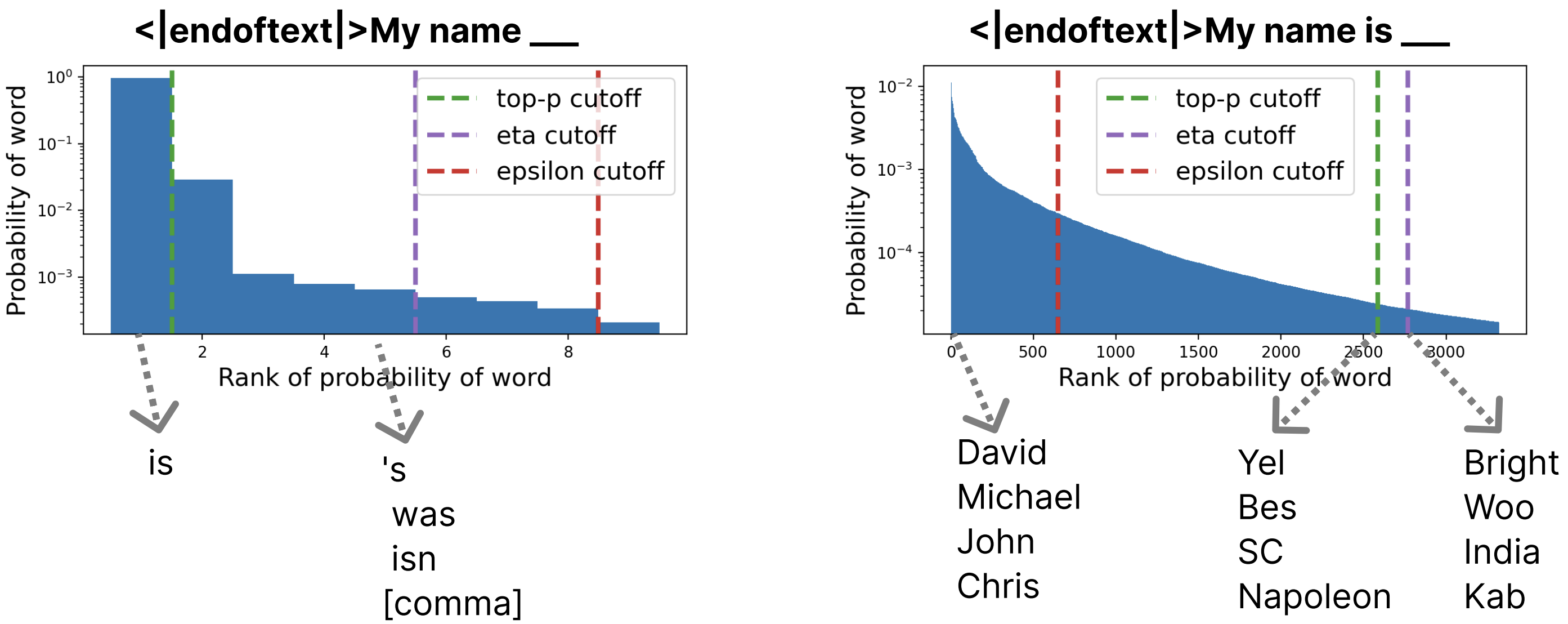
There are many ways to implement the “high probability is probably a good continuation; low-probability not so much” intuition. One very simple method is to just set some minimum threshold of probabilities for the accept set:
Intuitively, low probabilities are not just indicative of unlikely continuations, it's also just hard to estimate the probability of a thing whose true probability is very very low. This algorithm epsilon sampling (Hewitt et al., 2022) implements this intuition. There are some details here that one has to keep in mind however; for example, it is possible that no words are above the $\epsilon$ threshold, in which case often implementations will just generate the argmax word at that timestep.
By far the most popular truncation method is top-p sampling, also called nucleus sampling (Holtzman et al., 2020). The intuition of top-p sampling is that the most likely $p$ percent of the model's distribution at any timestep is “good” (should be kept) and the remaining $1-p$ lowest-probability percent is bad.
To interpret this, think of (1) sorting the vocabulary in decreasing order of probability, and then taking the $k$ most probable words such that $k$ is the minimal set whose sum of probabilities it at least $p$.
Each of these algorithms makes different assumptions about what is ``wrong'' about the distribution we've learned. Each also includes a parameter ($p$ or $\epsilon$) which controls the tradeoff of how much you cut of the distribution (which you'd like to avoid) vs how much you avoid potentially generating low-quality outputs (by cutting off the low-likelihood words.)
A final method we must discuss is temperature sampling, which is not a truncation sampling algorithm. It does not explicitly set any probabilities to zero; instead intuitively it interpolates in log space between the uniform distribution (arbitrarily high temperature) and the most likely token (zero temperature). The distribution is as follows:
Note the exponent — when $\tau$ approaches zero, logits are exponentiated, making the largest even larger relative to the others. When $\tau$ approaches infinity, logits are raised to the power of roughly $0$, so each gets probability roughly $\frac{1}{\mathcal{V}}$.