
Effectively all modern language model systems are based on reasoning models: language models that have been explicitly trained to generate a sequence of tokens before tey output their final answers. These tokens are variously called a thinking trace, or reasoning tokens, or a chain-of-thought, though the first two are sometimes used specifically to indicate that the model has been trained via reinforcment learning to perform said reasoning.
In this note we'll learn how to train a reasoning model, as well as how to think about the capabilities and limitations thereof.
So far in the class we've discussed the benefits of scaling the amount of computation we can put into training our models. To this end, we discussed pretraining and architectural parallelism, to spend floating-point operations to learn from text.
Another axis along which we can spend computation in order to achieve better performance is at test-time, or deployment time. That is, when a user asks a query, we want to be able to have a model (or system) “think harder” in order to better tackle a problem.
A simple way to implement this is to sample multiple answers in parallel, and then aggregate somehow. Concretely, consider a model we've trained to sample $\hat{y} \sim p_\theta(y\mid x)$, where $x$ is a mathematical lemma and $\hat{y}$ is an attempted proof of that lemma. What we've done so far is just sample once:
and we return the one sample $\hat{y}$.
Instead, we could sample $k$ times, with $k$ different seeds, to generate independent samples:
Now we have $k$ possible responses, and we can't return all $k$, so we have to aggregate—use the set of $k$ to choose a single response. The easiest case here is if we have a verifier—like how sometimes in mathematics, we can automatically check the correctness of a proof (say, if it's in Lean,) or maybe it's a set of test cases. A verifier is a function $v(x,\hat{y})$ such that:
So, our aggregation is simply to walk over all $k$ samples and return the first one that passes our verifier. Something like
though, it doesn't matter in this case which correct answer we return. If we don't have a verifier, we might instead use some heuristic for deciding betewen the $k$. For example, we might try to find a consensus candidate answer: the $\hat{y}_i$ most like the others that we generated (Wang et al., 2023). If we let $\phi(\hat{y})$ be a representation of $\hat{y}$ under the Transformer language model that generated it (say, some representation somewhere in the network), then we might use that for our aggregation:
So here, we're using representation similarity to compute which $y_i$ is most like the others.
Why might this work?
The intuition here is that if the model is good but sometimes makes mistakes, sampling multiple times and then choosing a consensus prediction may reduce the chance we return one of the bad samples (since, say, most samples are good.)
One problem with sampling many possible answers to a question is that none of them may be right, in which case no aggregation strategy will help. The problems we're trying to solve may be too difficult to solve directly; much like any hard problem, it may be necessary to work through intermediate problems, think it through, etc. A natural way to do this in a language model is to first tell it to do so (instruction following!) and then allow it to first generate tokens before its answer (Wei et al., 2022).
Consider the following input transformation: for an input sequence $x\in\mathcal{V}^*$, we'll simply prepend the sequence of tokens corresponding to our command:
With that now defined, we'll split the generation into two portoins: the chain of thought, and the answer. (This can be done, e.g., by adding special delimiter tokens, or just XML tags in plain text, like <think> and <\think>:
From here on we'll denote model outputs as follows:
which, recall, we can write equivalently as $\hat{y}, \hat{c} \sim p_\theta(y,c\mid x)$.
What makes a good chain of thought?
Well, to a first approximation, whatever makes the model come to a correct answer.
When we prompt the model to think step by step, we certainly hope the model's chain of thought will be helpful (and it is!) but if we want even better chains of thought, we might try training the model to do so. We begin this with simple supervised finetuning, on a dataset of inputs, chains of thought, and corresponding outputs $\mathcal{D} = \{(x_i, c_i, y_i)\}_{i=1}^{n}$:
where note that we are maximizing the likelihood of both the traces and the corresponding answers (so, our loss mask masks out only each $x_i$.)
Note as well here that we are training the model to generate chains of thought even when not prompted to! That is, in our SFT data, our $x$ are not $x_{\text{cot}}$; they don't have a prompt to think step by step. Instead, after this SFT, the default behavior of the model will be to think first and then answer.
tbd
So, how can our SFT fail to get us the behaviors we want?
A few ways.
For very hard problems, it's possible that we don't even know a useful chain of reasoning that gets us to the problem. But for now, let's assume this isn't an issue.
Another issue is that the model is being trained to perform behaviors during SFT that it will find difficult to perform on new problems. Here's an intuition. To solve difficult problems, you have to follow reasoning steps you understand, so you can apply then in new scenarios. If a tutor teaches you a few examples that use methods that are unfamiliar to you, it may be difficult for you generalize. If instead a tutor gives you examples that use methods that you yourself are already familiar with, you're much more likely to be able to apply them elsewhere. Not only this, but as you improve, you want the examples you're learning from to improve with you — if they don't that may limit your growth.
The language we use to discuss these things we often call on-policy vs. off-policy behaviors. We won't necessarily use this language, but you'll see it around so you need to know it. A sequence is on-policy simply if is drawn from the distribution defined by the model. So, if $\hat{y},\hat{c}\sim p_\theta(y,c\mid x)$, then $\hat{y}$ and $\hat{c}$ are on-policy for $p_\theta$. If not, then they're off-policy. Now, if some gave you a single sequence, say $c'$, and a model $p_\theta$, could you tell if $c'$ is on-policy for $p_\theta$? Not without a bunch of work; it's not obvious from just, say the likelihood $p_\theta(c')$. But if, say, you have some dataset you constructed somehow other than sampling from the model (like in the reasoning SFT we talked about just now,) then it's off-policy.
So, we want a way to train models to reason better in an on-policy way, to better hope that they generalize. For this, we'll come back to verifiers.
When we constructed our SFT dataset of reasoning, we had some method, maybe human evaluation, maybe some expensive process, of determining that indeed for input $x$, the reasoning trace $c$ and the answer $y$ are good or expected. But if we want on-policy learning of reasoning, all we have are maybe an input $x$, possibly an expected output $y$, and no notion of what the right reasoning trace $c$ is. This brings us back to the intuition that the right reasoning trace is whatever gets the model to the right answer, which we'll check with a verifier.
It's an old adage in computer science that verifying the correctness of an answer is (probably) easier than generating a candidate answer. A simple example of a verifier might just check that the answer is correct, so
This works when there is roughly one potential correct answer to the given question.
For example, in simple maths word problems, like Iroh has ten cabbages and gives half to Zuko..., there's a single integer answer, leading to easy verification. In something more complex like code, we might instead have a verifier that checks all the test cases; for tests $t_1,\dots,t_q$, we might have:
which we'd run in a container computing environment.
So, if we have a verifier, we have a way of telling whether our model's reasoning traces are good—if they lead to answers that are right. Here's a simple way to train the model to then generate more such reasoning traces:
We take our dataset $\mathcal{D}=\{(x_i)\}_{i=1}^{n}$ of just input problems, we sample a reasoning trace and answer for each, and then just train on the ones we got right:
So, is this on-policy learning?
Well, for the first gradient step it is, but then afterwards, it's not.
Let's make this clearer.
We sampled all of our reasoning traces and answers first, before we did made any updates to our parameters. Let's call that initial model $p_{\theta_0}$, indicating our initial model, while $p_\theta$ will refer to the “current” model throughout the optimization. So, we're working with:
Note how the expectation we're taking is with respect to the initial model, not with respect to the current parameters, so as we keep finetuning the model, we stray further from the distribution from which we sampled the sequences.
We want to instead maximize the likelihood of generating high-reward responses:
a traditional reinforcement learning goal.
Let's start with a simple way to try to solve our reinforcement learning problem: for each problem $x$, we just sample a batch of $k$ guesses (like we did when we were doing parallel sampling before!), compute the reward of each of them, and normalize the reward by the average reward of the batch. That is, we compute:
but we use $\bar{r}$, the normalized rewards for optimization, and then our gradient step is of the form:
Intuitively, look how we're (1) always sampling from the up-to-date model, and (2) basically performing SFT weighted by how much better than average the reward of each guess is.
GRPO (Shao et al., 2024) is a lot like our simple grouped reward algorithm. The first change is that our normalized reward will also correct for the standard deviation across a batch:
The second change is the introduction of the following importance sampling term. We consider taking multiple gradient steps on a single batch of data (or having our log-likilhoods at backpropagation time being different from those at sampling time, which can happen due to prefill-vs-sampling differences in numerical realities on the GPU,)
Note how for any function $f(x,y)$ if I take the expectation over (that is, sample according to) $p_{\theta_{\text{old}}}$ and reweight by $q$, then it's as if I'm taking the expectation over my real $p_\theta$:
Note how this has been done at the per-token level. These are importance sampling weights.
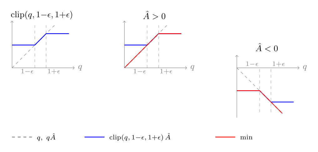
But, if our probabilities are too different, we don't want our importance sampling weights to be crazy. We do this through clipping. For a specific token $\hat{y}_{i,t}$, without clipping we'd be maximizing, in expectation:
where $\bar{r}(\hat{y}_i, x)$ is our normalized reward; often called $\hat{A}(\hat{y}_{i,t}, x)$ the advantage (and sometimes is dependent on the token; here our rewards are for the whole output, they don't differ per token.) The importance sampling ratio may be greater than or less than 1, so we clip the importance sampling ratio to a range between $1-\epsilon$ and $1+\epsilon$. Then the advantage may be greater than or less than zero, and so to be conservative, we take the minimum of the clipped and unclipped importance sampling-weighted advantage:
To get a visual intuition of the clipping, here are some LLM-generated nice plots of the different possibilities of advantage, importance sampling ratio, and clipping, which are a lot like Figure 1 in Schulman et al., 2017, which introduced the clipping for PPO, with some extra explanation:
Finally, here's GRPO, which again is a lot like simple grouped reward, but with the clipping and importance sampling ratios: