Eigentutorial

Before You can Use the Tool... If you're like me, you want to learn about the whole "eigen"-thing because it's used in a technique that you wish to understand. Unfortunately, that's a bad way to learn it. Eigenvectors and eigenvalues are like happiness; you cannot get it if you go directly after it. Before you can use the tool, you have to understand its underlying fundamentals. What are Eigenvectors and Eigenvalues? Let A be an n by n matrix. An eigenvector x of A is nothing but a (nonzero) vector that keeps its direction when multiplied by A. Its length can change (say, by λ), though. This λ is the eigenvalue of x. The picture you should have in mind is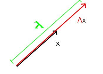 In equation, this would be just . That's it, nothing more. Before we do anything, let's figure out how to actually calculate the eigenvector x and eigenvalue λ (of A). As always, the beautiful aspect of computation is that we have to be absolutely precise. In Least Squares Approximations, we found a way to compute the projection (the "shadow") by exploiting the property of orthogonality: two vectors are orthogonal if their dot product is zero. Here, we exploit an analogous fact that a matrix has no inverse iff its determinant is zero. Solving the last equation boils down to finding roots of a polynomial in λ of degree n (we'll always find some root if we allow complex numbers). So we'll have several eigenvalue λs. For each λ, plug it into the second equation (A-λI)x = 0 to solve for the associated eigenvector x. Note the matrix A-λI is singular and consequently there are infinitely many solutions for x. This makes sense because if x retains its direction when multiplied by A, any vector in this direction is an eigenvector. Typically, you'll have n independent eigenvectors; don't allow me to diverge to cases you don't. 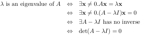What Do We Care for? Answer: decomposition. Just like orthogonality, this abstract notion of invariant direction reveals the structure of the matrix A. The eigenvectors, with their fixed directions, serve as the axes of the world defined by A. That's what we care for when anything comes to eigenvectors and eigenvalues. 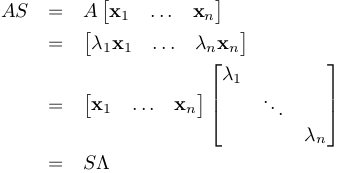The simplest decomposition happens when A is n by n and has n independent eigenvectors (as assumed so far), because if S is an n by n matrix having the eigenvectors x_1...x_n as columns, and Λ (the capital λ) is an n by n diagonal matrix having the corresponding eigenvalues λ_1...λ_n as entries, we find that 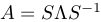Thus the "eigendecomposition" is possible (S is invertible since its columns are independent). We also say A is diagonalized (into the diagonal eigenvalue matrix Λ). Another way to view this is to think of Λ as an "eigenmatrix" whose "direction" is never changed: . 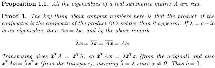A more powerful decomposition happens when A is a real symmetric matrix. Why? Well, first off, all the eigenvalues of A are real. 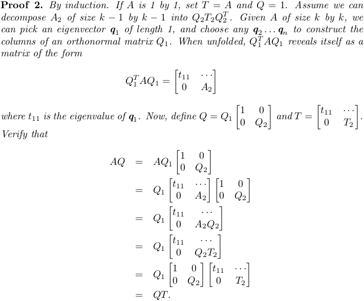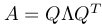Second, it can always be diagonalized. To see this, we need a lemma. The proof requires some trick (as shown in Strang's textbook): When A is (real) symmetric, T has to be symmetric as well as upper triangular, meaning diagonal, with eigenvalue entries. This shows why the decomposition is so nice for a real symmetric matrix A. For such A, can be done with a real eigenvalue matrix Λ and an orthonormal eigenvector matrix Q. This symmetric diagonalization is called the Spectral Theorem. What if A is not Square? So far, we've talked about finding direction-invariant eigenvectors where we simply observe . But in general, A is not square, but rather of size m by n where m is not equal to n. No vector will survive the application of A in its original dimension, so that observation is no more valid. We still want to find a defining set of vectors of A. What do we do? 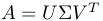Answer: the Singular Value Decomposition (SVD) In my opinion, there are two related but vastly different ways to understand the SVD, and it's best to keep them cleanly separated. The first is the practical one: it's a method to solve the above "non-square A decomposition" problem, by treating the two sides of A as two views of the same matrix. This motivates the second way to understand the SVD: it's a method to find orthonormal bases for all the four fundamental subspaces of A (the row, column, null, and left null space). Let's stick to the former in this tutorial; I was confused to see these two ways, however related, jumbled together. Two Views of the Matrix OK, the eigenvector will not survive the multiplication by A, because its dimension will change from n to m. But what if we treat the row space (in ) and the column space (in ) as two different spaces from which to look at A? We postulate that no matter what space we're in, the defining vectors of A will be more-or-less the "same". Indeed, we're strongly convinced we're right, because the Fundamental Theorem of Linear Algebra tells us that the dimension of both the row and the column space is the rank of A (call it r). (***) Thus we tentatively attempt to find the pairs of vectors and (where and ) such that . Furthermore, we'd like to have that U = [u_1...u_r] and V = [v_1...v_r] orthonormal (U'U = I and V'V = I) to serve as the basic skeleton of A. We call and the singular vectors and the associated the singular values of A. As in the case of the simple "eigendecomposition", this will allow us to say . 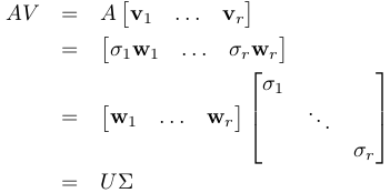So we'll have , and our goal will have been accomplished. That was the motivation. Now, the hard part is, how do we find such vectors and values, let alone knowing whether they exist? The intuition is that u's should be normalized projections of orthogonal v's: 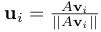(which makes u's orthonormal). That way, each singular value σ is simply the length of the projection, ||Av||. If this is the case, the only unknown is v; once we know how to compute v, everything else falls along. 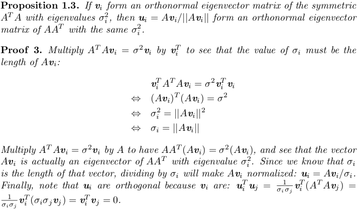How to find v? The key is to note that A may not be square, but A'A is (n by n). Not only that, it is also symmetric, because (A'A)' = A'(A')' = A'A. By the Spectral Theorem, we can always find an orthonormal eigenvector Q that decomposes A'A into QΛQ'. So we multiply by A' to the left, removing U in the process by its orthonormality: A'A = (UΣV')'(UΣV') = (VΣ'U')(UΣV') = V(Σ'Σ)V'. This shows V can be found as the orthonormal eigenvector matrix of A'A, along with Σ'Σ as the eigenvalues. We can do exactly the same thing by looking at AA' (m by m): AA' = (UΣV')(UΣV')' = (UΣV')(VΣ'U') = U(ΣΣ')U', arriving at the conclusion that U can be found as the orthonormal eigenvector matrix of AA', along with ΣΣ' as the eigenvalues. A few facts from this observation are: The eigenvalues of A'A and AA' are the same. Each eigenvalue must be the square of the corresponding singular value: σ^2. v's are the orthonormal eigenvectors of A'A. u's are the orthonormal eigenvectors of AA'. The most important message is that thanks to the Spectral Theorem, it is always possible to find the singular vectors v's and u's, along with their singular values σs, such that they have the properties we desire in diagonalizing a non-square matrix (***). Now we prove this result that we've reached by intuition. . 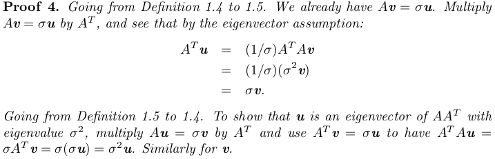Caveat: Two Definitions for Singular Values The way we have reached the singular values is to view them as the squared roots of eigenvalues. . But Wikipedia defines it as follows: . Did I lie? No. Claim: The above two definitions of singular values are equivalent. The latter just happens to be applicable more frequently. Summary, Implications, and Conclusion The SVD says that given any m by n matrix A of rank r, we can decompose it into A = UΣV'. U = [u_1...u_r] and V = [v_1...v_r] are simply orthonormal eigenvectors of AA' and A'A. Each pair u_i and v_i have the same eigenvalue λ_i. The r by r diagonal matrix Σ will contain singular values σ_i = sqrt(λ_i). In other words, A is decomposed into rank 1 matrices u_iσ_iv_i' --- total r components. A = UΣV' = u_1σ_1v_1' + ... + u_rσ_rv_r'. When σ_i is ordered so that σ_1 >= σ_2 >= ... σ_r > 0, can interpret the r matrices u_1σ_1v_1',...,u_rσ_rv_r' as the "pieces" of A in order of importance, because u_i and v_i are the joint direction-invariant axes of A from different views that agree on their "importance" σ_i. This is a powerful way to discover the structure of any matrix. It's also unsupervised (i.e., no external help). Any component analysis (principal, canonical, etc.) is almost a direct translate of this result. We'll soon have a glance at these applications.