Thou art Orthogonal
The power of linear algebra is in visualizing the vectors so that we may exploit the physical geometry of the system to immediately get the answer. Orthogonality (A prototypical illustration of orthogonality is the Least Squares Approximations (LSA). I never liked that name. It comes up often, but what does that even mean? Sounds complicated! Strang's textbook gives an excellent presentation on LSA, but I'll try to make it more fun and intuitive.
LSA: Reach for the Unreachable Solution
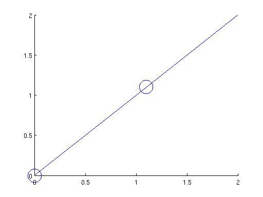
Let's get the obvious question out of the way. What does that name LSA mean? In its full version, it stands for "Using the orthogonality of vectors to give Least Squared length of the error vector in your Approximations of the solution".Why do we even need to resort to approximations? Suppose you want to find a linear function f (in real) that satisfies certain conditions. You might say, "It can be whatever, but I want it to spit out 0 on 0 and 1.1 on 1.1". In this case, there is a unique f that grants your wish, namely f(x) = x.
 .
.
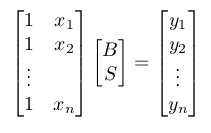
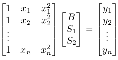
This is just Ax=b if we define 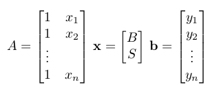 .
.
Let's look at A, which is an nx2 matrix. The rank (:= the number of "pivots", or the head of nonzero rows
after forward elimination) of A is going to be at most 2. The Fundamental Theorem of Linear Algebra then tells us that
the space spanned by the two columns of A can have dimension at most 2. If we were to have an exact solution
for x, b must be in this column space, but it is unlikely that b will be in such a small space if n > 2.
(Of course, the best scenario is A is square and invertible so that we can simply compute
![]() , but that's out of question as soon as you have more than two equations to satisfy.)
, but that's out of question as soon as you have more than two equations to satisfy.)
Now that we know we don't have an exact solution, no matter what B and S we pick for x, Ax is not going to be equal to b and consequently the error e = b - Ax is going to be nonzero. How do we make the error as small as possible? This is where visualizing vectors is useful.
Projection: Follow the Shadow
Ordinarily, when we have two vectors v and w, we want to somehow relate them. A good way is to "project" one (say v) onto the other, and examine the "shadow" p of v on w.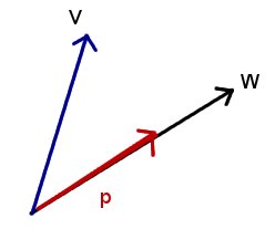
Lemma: two vectors v and w are orthogonal if their dot product is zero.
Proof: ![]() by geometry;
only the element-wise product of v and w remains as 0 after the dust settles.
by geometry;
only the element-wise product of v and w remains as 0 after the dust settles.
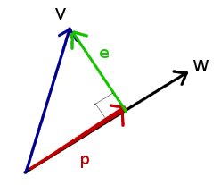
In other words, finding a such that
e = w - p = b - aw and
w are orthogonal means finding a such that:
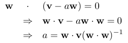 . What a nice closed form!
The situation is exactly the same when we project onto a subspace A instead of w;
the multiple will be a vector x instead of a scalar a, and the solution is
. What a nice closed form!
The situation is exactly the same when we project onto a subspace A instead of w;
the multiple will be a vector x instead of a scalar a, and the solution is
![]() (the "dot product" of two matrices is simply
the product with the left one transposed--I'll use A' to express A transposed).
(the "dot product" of two matrices is simply
the product with the left one transposed--I'll use A' to express A transposed).
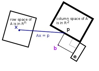
Coming back to our original task, we wish to find a 2x1 vector  such that
the error e = b - Ax is minimized. In light of the above exploration,
we project b onto A because the "shadow" will give us the projection Ax that is
"closest" to b (keep in mind that b is an n-dimensional vector, so it's hard to visualize).
The important picture below is given by Strang, and it's well worth studying carefully.
such that
the error e = b - Ax is minimized. In light of the above exploration,
we project b onto A because the "shadow" will give us the projection Ax that is
"closest" to b (keep in mind that b is an n-dimensional vector, so it's hard to visualize).
The important picture below is given by Strang, and it's well worth studying carefully.
The Solution
We can't solve Ax = b exactly. But we know the vector Ax closest to b comes from the x that yields the error vector b - Ax orthogonal to A, implying A'(b - Ax) = 0. This gives A'Ax = A'b, and thus x = (AA')^{-1}A'b is the bias and slope we want for the function f. The only condition for AA' to be invertible is that the two columns are independent, so we're safe. When we expand A'A and A'b in A'Ax = A'b, we come to the conclusion that the line defined by x = (B,S) minimizes the error when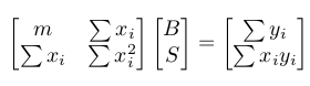 .
.
Final Jump: Now now now... Where does the "least squares" come in? This choice of x minimizes
the squared length of Ax - b (how much we screw up) because this vector is the hypothenuse
of the right triangle formed by Ax - p and e;
Ax - p, being in the column space, has to be orthogonal to e,
which is in the left null space. This gives us
![]() , where we note that the length of Ax - p can
only be positive and therefore Ax - b is minimized by choosing Ax = p.
, where we note that the length of Ax - p can
only be positive and therefore Ax - b is minimized by choosing Ax = p.
Calculus approves! Minimizing the squared length ![]() by differentiating with respect to B and S results in the system of equations
by differentiating with respect to B and S results in the system of equations
,Demonstration
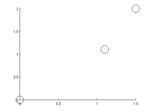
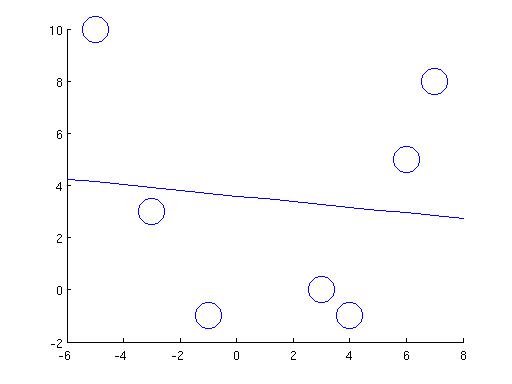
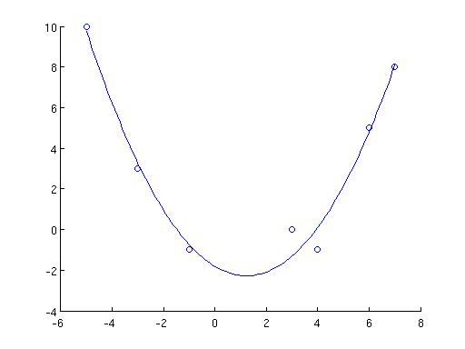
Does it work? Well, for the example in the beginning, we couldn't fit the three points (0,0), (1.1,1.1), and (1.5,2) with a straight line. This one-liner in matlab,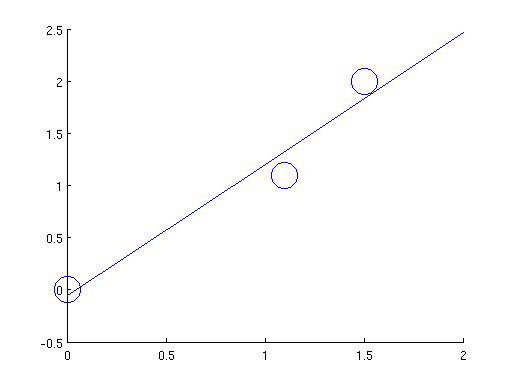
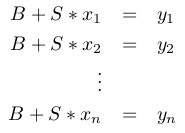
1. We want to find B, S(1), and S(2) such that the following is satisfied:
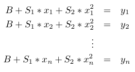
 .
.
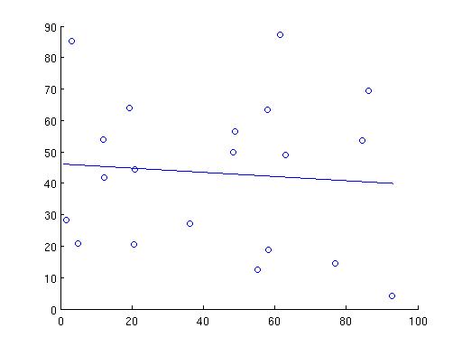
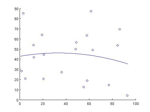
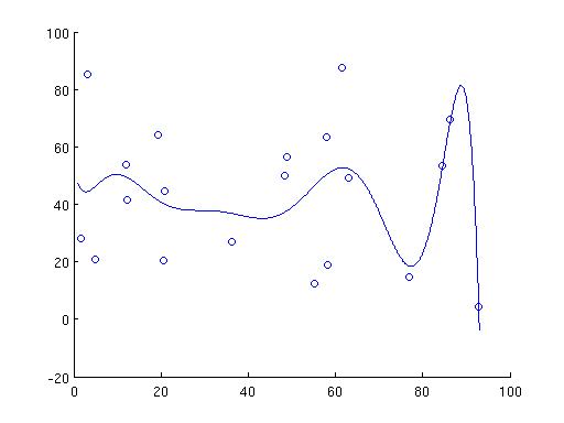
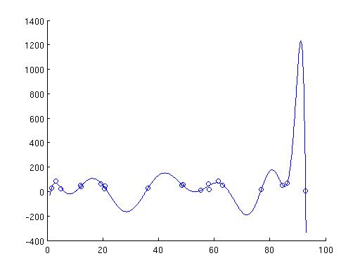
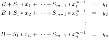
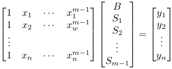
In fact, while at it, let's make it fully general. We fit a polynomial of power m-1 to the points. When m=2, it is a straight line. When m=3, it is a parabola. The new definition of nxm A and mx1 x is driven by the following goal:
1. We want to find B, S(1), ..., S(m-1) such that the following is satisfied:
 .
. .
.