Conditional and Unconditional Bayesian Integration

In this appendix, we carry out the result shown earlier relating the Bayesian estimation of conditional and joint densities. In presenting these two inference problems, we discussed how they might lead to different solutions despite the fact that they both involve exact techniques (integration and conditioning). In addition, some speculation about the superiority of the direct conditional estimate was made. In the following, we present a specific example to demonstrate this difference and to argue in favor of the conditional estimate p(y|x)^c versus the conditioned joint estimate p(y|x)^j.

To prove this point, we use a specific example, a simple 2-component mixture model. Assume the objective is to estimate a conditional density, p(y|x). This conditional density is a conditioned 2-component 2D Gaussian mixture model with identity covariances. We try to first estimate this conditional density by finding the joint density p(x,y) and then conditioning it to get p(y|x)^j. Subsequently, we try to estimate the conditional density directly to get p(y|x)^c without obtaining a joint density in the process. These are then compared to see if they yield identical solutions.

  

Figure 11.1: 2D Mixture Model

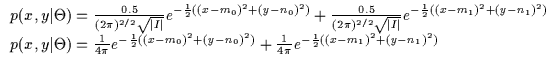
Consider a joint density as a two-element 2D Gaussian mixture model with identity covariance and equal mixing proportions shown in Figure 11.1. We wish to fit this model to data using Bayesian integration techniques. The result will not be significant on its own since this is a trivial learning example. However, we shall check for inconsistencies between this result and direct conditional density estimation to prove a general statement about Bayesian inference. Equation 11.1 depicts the likelihood of a data point (x,y) given the model and Equation 11.2 depicts a wide Gaussian prior (with very large $\sigma^2$) on the parameters (m₀, n₀, m₁, n₁). As shown earlier, we wish to optimize this model over a data set $({\cal X},{\cal Y})$. This computation results in a model p(x,y) as in Equation 11.3.

 

$$\begin{array}{l} p(x,y\vert\Theta) = \frac{0.5}{(2\pi)^{2/2} \sqr... ...)^2)} + \frac{1}{4\pi} e^{-\frac{1}{2} ((x-m_1)^2 + (y-n_1)^2)} \\ \end{array}$$ (11.1)

 

$$\begin{array}{l} p(\Theta) = \frac{1}{(2\pi)^{4/2} \sqrt{\vert\si... ...^{-\frac{1}{2\sigma^2} ((m_0)^2 + (n_0)^2 + (m_1)^2 + (n_1)^2)} \\ \end{array}$$ (11.2)

 

$$\begin{array}{ll} p(x,y) & = p(x,y\vert{\cal X},{\cal Y}) \\ & =... ...{N} {\rm choose}_\sigma [ \gamma , \omega ]_i } dm_0 dn_0 dm_1 dn_1 \end{array}$$ (11.3)

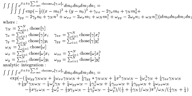
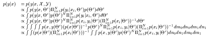
In Equation 11.3 we are effectively summing over all the permutations $\sigma$ of the assignments of the N data points to the 2 different models. For each $\sigma$, we select a different assignment of the i data points. Each point gets assigned to one of 2 Gaussians (one related to $\gamma$ and the other related to $\omega$). The summation over the data in each exponential can be further simplified as in Equation 11.4 and then analytically integrated. The integrals are summed over all possible assignments of the data points to one of the two Gaussians (i.e. M^Npossibilities or integrals where M=2 models here). Essentially, we are iterating over all possible permutations where the data points are assigned to the two different Gaussians all 2^N different ways and estimating the Gaussians accordingly. Evidently this is a slow process and due to the exponential complexity growth, it can not be done for real-world applications. Figure 11.2 shows some data and the Bayesian multivariate mixture model estimate of the probability density p(x,y). Figure 11.3 shows the conditional density p(y|x)^j.

  

Figure 11.2: Joint Density Estimate

 

$$\begin{array}{l} \int \int \int \int e^{\beta + \delta + \sum_{i=... ...) / \omega_N) \pi^2 / \omega_N / (\frac{1}{4} \gamma_N+\frac{1}{4}) \end{array}$$ (11.4)

  

Figure 11.3: Conditioned Joint Density Estimate

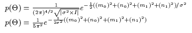
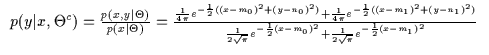
By solving another integration, we can directly compute the conditional density p(y|x)^c. The conditional density has the form shown in Equation 11.5. This is just a regular 2-component conditioned mixture of Gaussians model with identity covariances. Assume that we are using the same prior as before. In addition, note the presence of the exact same parameters m₀, n₀, m₁, n₁ which reside in the conditioned parametrization of $\Theta$which can be called $\Theta^c$.

 

$$\begin{array}{l} p(y\vert x,\Theta^c) = \frac{ p(x,y\vert\Theta)}... ...}{2}(x-m_0)^2} + \frac{1}{2\sqrt{\pi}} e^{-\frac{1}{2} (x-m_1)^2} } \end{array}$$ (11.5)

The resulting Bayesian integration is depicted in Equation 11.6. Unfortunately, integration can only be completed analytically for the parameters n₀ and n₁. Thus, the integration over the other 2 parameters is performed using numerical approximation techniques. The inner integral of n₀ and n₁ causes the exponentially complex assignment permutation seen above and this is compounded with the computation of the integral numerically by a grid approach. This is therefore an even more cumbersome computation than the joint density Bayesian estimate and is only shown here as an example. There exist more efficient numerical integration techniques such as superior quadrature approaches or Monte-Carlo methods however this Bayesian integration approach is typically too intensive for any real-world applications. It should be noted that typically, Bayesian density estimation, Bayesian sampling techniques and Bayesian integration are quite cumbersome except in very special situations.

 

$$\begin{array}{ll} p(y\vert x) & = p(y\vert x,{\cal X},{\cal Y}) \... ...heta^c)^N \Pi_{i=1}^{N} p(x_i,y_i\vert\Theta^c) dn_0 dn_1 dm_0 dm_1 \end{array}$$ (11.6)

  

Figure 11.4: Direct Conditional Density Estimate

The same data is thus fitted with the conditional model which produces the conditional distribution p(y|x)^c shown in Figure 11.4. Surprisingly, this is quite different from the conditioned joint density. In fact, if we consider a slice of the conditional densities at an arbitrary x value, we obtain the y-distributions shown in Figure 11.5. This indicates that the directly computed conditional model was able to model the bi-modal nature of the data while the conditioned joint density model was not. In fact, p(y|x)^c seems like a better choice than p(y|x)^j.

  

Figure 11.5: Slices of p(y|x)^j and p(y|x)^c at x = -5

The above suggests the following. Consider the case of two Bayesian statisticians (A and B) who are asked to model a conditional density (i.e. in a classification task or a regression task) from data. Statistician A assumes that this conditional density arises from a joint density. He then estimates this density using full Bayesian inference. He then conditions this joint density and obtains the final conditional density he was asked to produce. Statistician B assumes nothing about the origins of the conditional density and estimates it directly. He only uses a parametric form for a conditional density, it is just a function. At the end of the day, the two have different models even though all the manipulations they performed where valid equalities (Bayesian inference and conditioning are exact manipulations). Thus, by a strange by-product of the paths the two statisticians took, they got two different answers: $p(y\vert x)^c \neq p(y\vert x)^j$. Typically p(y|x)^c seems to be a more robust estimate and this is probably because no extra assumptions have been made. In assuming that the original distribution was a joint density which was being conditioned, statistician A introduced unnecessary constraints ^11.1 from the space of p(x,y) and these prevent the estimation of a good model p(y|x). Unless the statisticians have exact knowledge about the generative model, it is typically more robust to directly estimate a conditional density than try to recover some semi-arbitrary joint model and condition it. Figure 11.6 graphically depicts this inconsistency in the Bayesian inference shown above. Note here that the solutions are found by fully Bayesian integration and not by approximate MAP or ML methods. Thus, the discrepancy between p(y|x)^j and p(y|x)^c can not be blamed on the fact that MAP and ML methods are just efficient approximations to exact Bayesian estimation.

  

Figure 11.6: Inconsistency in the Bayesian Inferences