Placing and Tightening the Bound

In general, a lower bound has many parameters which allow it to support the function being optimized in different ways. We outline three desiderata that should be followed for placing the lower bound on the function. Typically, when we shall use bounding techniques in this document and when we discuss their further properties, we shall assume that these requirements are being met whenever possible.

• Requirement 1 $\longrightarrow$ Contact

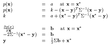
  The bound must make contact with the function (Equation 6.4) at the current operating point for the maximization process to behave as described earlier.

  
  

   

  $$\begin{array}{l} p({\bf x}) \leq f({\bf x}) \:\:\:\: \forall {\bf x} \\ p({\bf x}^*) = f({\bf x}^*) \end{array}$$ (6.4)

  
  

• Bound Requirement 2 $\longrightarrow$ Tangentiality

  The bound's tangent plane should be parallel to the function's tangent plane at the current operating point as in Equation 6.5. Otherwise, there will be an intersection between the function and the lower bound and the lower bound will rise above it, violating the lower bound assumption.

  
  

   

  $$\begin{array}{l} \frac{\partial p({\bf x})}{\partial {\bf x}} = \... ... x}} \:\: \rm {at} \:\: {\bf x} = {\bf x}^* \epsilon {\cal R}^n \\ \end{array}$$ (6.5)

  
  

• Bound Requirement 3 $\longrightarrow$ Tightness

  Finally, the bound should be as 'close' to the function as possible to approximate the function properly. Typically, a lower bound which falls away from the function too quickly is not very likely to cause rapid optimization. In other words, what is desired is that the maximum of the bound is close to the maximum of the function. Let us focus on the quadratic bound described earlier (Equation 6.6).

  
  

   

  $$\begin{array}{ll} p(x) = k - \frac{(x-y)^2}{\sigma} & x \epsilon ... ...y})^T \Sigma^{-1} ({\bf x} - {\bf y}) & {\bf x} \epsilon {\cal R}^n \end{array}$$ (6.6)

  
  

  We use ${\bf y}$ to denote the location parameter which moves the locus of the parabola's maximum around. The k parameter varies the maximum's amplitude. Finally, note the $\Sigma$ (or $\sigma$ in 1 dimension). This is the scale (or shape) parameter which changes the shape and orientation of the parabola. We can also define the inverse of the scale parameter as $W = \Sigma^{-1}$ (or $w = \frac{1}{\sigma}$).

  Typically, the scalar parameter k and the location parameter ${\bf y}$ are determined directly from the constraints in Equation 6.4 and Equation 6.5. However, the scale parameter remains to be determined. Evidently, it must be chosen so that the lower bound property of the quadratic is not violated. However, we also would like to maximize the determinant of the scale parameter as given by Equation 6.7.

  
  

   

  $$\begin{array}{l} \max \vert \Sigma \vert \:\:\: {\rm s.t.} \:\:\:... ...{-1} ({\bf x} - {\bf y}) \:\:\: \forall {\bf x} \epsilon {\cal R}^n \end{array}$$ (6.7)

  
  

  This statement is not as obvious as the previous two requirements and we justifiy it subsequently.

  
  

   

  $$\begin{array}{l} p({\bf x}) \leq f({\bf x}) \:\:\:\: \forall x \\... ...l {\bf x}} = {\bf b} \:\:\: \:\:\:{\rm at} \:\: {\bf x} = {\bf x}^* \end{array}$$ (6.8)

  
  

  Suppose that Requirements 1 and 2 have been resolved and, specifically, we have the computed Equation 6.8 to obain real values (a and ${\bf b}$). These expressions can be manipulated further for the case of the quadratic as in Equation 6.9 yielding two constraint expressions (containing the constant terms a and ${\bf b}$).

  
  

   

  $$\begin{array}{lll} p({\bf x}) & = & a \:\:\:\:\:\: {\rm at} \:\: ... ... = & {\bf b} \\ {\bf y} & = & \frac{1}{2}\Sigma{\bf b} + {\bf x}^* \end{array}$$ (6.9)

  
  

  The expressions in Equation 6.9 can then be used to isolate k and express it exclusively in terms of the constants ${\bf x}^*$, a and ${\bf b}$ as well as the still free shape parameter $\Sigma$. Note the isolated k in Equation 6.10 and its relationship to $\Sigma$ (or W equivalently). As we increase $\vert\Sigma\vert$ (or decrease |W|), we are effectively increasing k. The larger $\vert\Sigma\vert$ yields high values of k. Since maximizing the quadratic bound will move our current locus from ${\bf x}^*$ to ${\bf y}$ the higher the $k = p({\bf y}) \leq f({\bf y})$ the higher the value of the function we can jump to. It is obvious that the widest parabola or maximal $\vert\Sigma\vert$is desirable since it is more likely to allow higher jumps in the function being optimized. In reality, we would ideally like to maximize the expression ${\bf b}^T \Sigma {\bf b}$ over all the elements of the $\Sigma$. Thus the requirement for maximal $\Sigma$or maximal k can be interchanged.

  
  

   

  $$\begin{array}{lll} k & = & a + ({\bf x}^* - {\bf y})^T \Sigma^{-1... ...x^*} - {\bf y}) \\ k & = & a + \frac{1}{4}{\bf b}^T \Sigma {\bf b} \end{array}$$ (6.10)

  
  

  In fact, we typically begin by finding the optimal $\Sigma$^6.2 and then isolating the corresponding k and ${\bf y}$. These three quantities are really functions of the operating point ${\bf x}^*$ (once the function to optimize, f(), is specified of course) and can be expressed as functions of each other as well. This concept is demonstrated in concrete examples that will follow.