Object Recognition System

Since the video camera is aligned with the line of sight, by gazing at interesting objects, the user directs the input to the recognition system which tries to recognize previously recorded objects. The recognition results are then sent to the audio-visual associative memory system which plays the appropriate clip.

The generic object recognition system used by DyPERS has been recently proposed by Schiele and Crowley [Schiele and Crowley, 1996]. A major result of their work is that a statistical representation based on local object descriptors provides a reliable means for the representation and recognition of object appearances.

Objects are represented by multidimensional histograms of vector responses from local neighborhood operators. Simple matching of such histograms (using $\chi^2$-statistics or intersection [Schiele and Crowley, 1997]) can be used to determine the most probable object, independent of its position, scale and image-plane rotation. Furthermore the approach is considerably robust to view point changes. This technique has been extended to probabilistic object recognition [Schiele and Crowley, 1996], in order to determine the probability of each object in an image only based on a small image region. Experiments (briefly described below) showed that only a small portion of the image (between 15% and 30%) is needed in order to recognize 100 objects correctly. In the following we summarize the probabilistic object recognition technique used. The current system runs at approximately 10Hz on a Silicon Graphics O2 machine using OpenGL extensions for real-time image convolution.

Multidimensional receptive field histograms are constructed using a vector of any linear filter. Due to the generality and robustness of Gaussian derivatives, we selected multidimensional vectors of Gaussian derivatives (typically the magnitude of the first derivative and the Laplace operator at two or three different scales). In order to recognize an object, we are interested in computing the probability of the object O_n given a certain local measurement M_k (here a multidimensional vector of Gaussian derivatives). This probability p(O_n|M_k) can be calculated using Bayes rule:

$$\begin{eqnarray*}p( O_n \vert M_k ) &=& \frac{ p(M_k\vert O_n) p(O_n)}{ p(M_k)} \end{eqnarray*}$$

with p(O_n) the a priori probability of the object O_n, p(M_k) the a priori probability of the filter output combination M_k, and p(M_k|O_n) is the probability density function of object O_n, which differs from the multidimensional histogram of an object O_n only by a normalization factor.

Having K independent local measurements M₁, M₂, $\dots,$ M_Kwe can calculate the probability of each object O_n by:

 

$$p( O_n \vert M_1, \dots, M_k ) \frac{\prod_k p(M_k\vert O_n) p(O_n) } { \prod_k p(M_k) }$$ = (1)

M_k corresponds to a single multidimensional receptive field vector. Therefore K local measurements M_k correspond to K receptive field vectors which are typically from the same region of the image. To guarantee independence of the different local measurements we choose the minimal distance d(M_k,M_l) between two measurements M_k and M_l to be sufficiently large (in the experiments below we chose the minimal distance $d(M_k,M_l) \geq 2 \sigma$).

In the following we assume the a priori probabilities p(O_n) to be known and use $p(M_k) = \sum_i p(M_k\vert O_i) p(O_i)$ for the calculation of the a priori probability p(M_k). Since the probabilities p(M_k|O_n) are directly given by the multidimensional receptive field histograms, Equation (1) shows a calculation of the probability for each object O_n based on the multidimensional receptive field histograms of the N objects. Perhaps the most tempting property of Equation (1) is that we do not need correspondence. That means that the probability can be calculated for arbitrary points in the image. Furthermore the complexity is linear in the number of image points used.

  

Figure: Experimental results for 103 objects. Comparison of probabilistic object recognition and recognition by histogram matching: $\chi^2_{qv}$ (chstwo) and $\cap$ (inter). 1327 test images of 103 objects have been used.

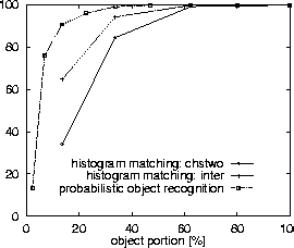
Equation (1) has been applied to a database of 103 objects. In an experiment 1327 test images of the 103 objects have been used which include scale changes up to $\pm 40$%, arbitrary image plane rotation and view point changes. Figure 4 shows results which were obtained for six-dimensional histograms, e.g. for the filter combination Dx-Dy-Lap at two different scales ( $\sigma = 2.0$ and = 4.0). A visible object portion of approximately 62% is sufficient for the recognition of all 1327 test images (the same result is provided by histogram matching). With 33.6% visibility the recognition rate is still above 99% (10 errors in total). Using 13.5% of the object the recognition rate is still above 90%. More remarkably, the recognition rate is 76% with only 6.8% visibility of the object. See [Schiele and Crowley, 1996,Schiele and Crowley, 1997] for further details.