Due: Thursday, April 10 at 11:59 pm
Submission: On Courseworks
Please read the instructions carefully. An incorrectly formatted submission may not be counted.
There are several questions in this assignment.
This assignment starts from skeleton code called nbody.py.
Please include comments in your code detailing your thought process where appropriate.
Put nbody.py in a folder called uni-hw7 (so for me this would be tkp2108-hw7).
Then compress this folder into a .zip file.
For most operating systems, you should be able to right click and have a “compress” option in the context menu.
This should create a file called tkp2108-hw7.zip (with your uni).
Submit this on courseworks.
In this homework, we will start working towards the implementation of our N-Body simulator. In this simulation, we will attempt to model the movement of a number of bodies interacting with and on each other. These simulations are applicable in fields like astrophysics, particle physics, and molecular dynamics, where a number of bodies in motion influence each other with gravitational, electromagnetic, and/or nuclear forces.
The motion of these bodies is dictated by continuous equations - that is, as each body moves, the forces induced by every other body are in flux, altering those forces and influencing the movement. Such equations are extremely difficult if not impossible to solve analytically, so exact solutions for the position of each body over the course of the interaction is impossible to solve as a pure function of time.
In the lectures we discussed simulations and how we can reduce the complexity of our math by freezing time and relying on the values of much simpler instanteneous equations over short time steps. In layman’s terms, rather than attempt to solve the above problem, we:
∆t, assuming the force is constant over that small interval∆t and repeatThus, instead of requiring very complicated analytic solutions, we can rely on the much simpler instantaneous equations (and accumulating some error in the process).
For the next two homeworks, we will be building a simulator to model an arbitrary number of objects in two dimensions. Each object will be randomly assigned a position, mass, and initial velocity. Using the equation for gravitational force we covered in the lectures on simulations, we will then simulate each objects motion over a certain simulation duration. Over the course of the simulation, we will collect statistics about what is going on during the simulation, and we will animate (in the form of a sequence of plots) the motion of our objects. The end result should look like a much more interesting and complicated version of the gif above.
Before we write the simulation, we will familiarize ourselves with some of the libraries and tools we will use, as well as the Physics required. In this first homework on N-Body simulations, we will get comfortable using numpy arrays and matplotlib plotting functionality.
Before we start performing calculations, lets come up with some representative data:
def generateObjects(count, center=0, width=10):
    """Generate a `count` x 5 matrix of (x, y) coordinates corresponding to `count` number of arbitrarily placed elements

    (x,y) coordinates should be generated according to a normal distribution.
    Mass should be randomly generated integer between 10 and 100.
    (vx,vy) velocities should be 0 for this homework.

    Args:
        count (int): the number of (x, y) pairs to generate
        center (int): the center of our distribution (average if `method`=normal)
        width (int): the width of our distribution (covariance if `method`=normal)

    Returns:
        a (`count`, 5) array of positions, mass, velocities

        The return value should look like:
            [[x1, y1, mass1, vx1, vy1],
             [x2, y2, mass2, vx2, vy2],
             ...
            ]
    """
Our generated numpy matrix should consist of count rows, each representing a body in space.
The first two elements of each row correspond to its x,y position in space.
This should be generated from a 2D normal distribution, e.g. a 2D bell curve, so that most of our objects are in the center.
Numpy has a convenient method for this, np.random.multivariate_normal.
The third element of each row should correspond to an object’s mass.
We should pick an number in range (10,100) for this to work nicely with our future animation code.
The final two elements are the objects' initial velocity in x and y dimensions.
For now, you can initialize these both to 0.
Later on, we will put a very large mass at the center of these objects, and give them all an initial rotational velocity to simulate a real-world rotating galaxy.
To test your code, all this function and inspect the results.
X/Y values should lie width round the origin, and masses should be between 10 and 100.
Once we can plot, we can further validate that our distribution looks like it should.
objects = generateObjects(10, center=0, width=100)
print(objects)
array([[-1.98395882e+00, -1.16473183e+00,  4.30000000e+01, 0.00000000e+00,  0.00000000e+00],
       [ 1.58399159e+01,  8.16913289e+00,  8.10000000e+01, 0.00000000e+00,  0.00000000e+00],
       [-6.69012470e+00, -9.48339048e+00,  8.10000000e+01, 0.00000000e+00,  0.00000000e+00],
       [-1.19430673e+01,  2.28630302e+01,  3.30000000e+01, 0.00000000e+00,  0.00000000e+00],
       [-3.94048371e+00, -1.99088897e-02,  4.80000000e+01, 0.00000000e+00,  0.00000000e+00],
       [-7.32319077e+00, -5.54311988e+00,  2.30000000e+01, 0.00000000e+00,  0.00000000e+00],
       [ 1.49400991e+01,  7.53181500e+00,  1.40000000e+01, 0.00000000e+00,  0.00000000e+00],
       [ 1.59951768e+01,  3.25613984e+00,  5.00000000e+01, 0.00000000e+00,  0.00000000e+00],
       [-1.00611716e+01, -8.88840857e-01,  7.80000000e+01, 0.00000000e+00,  0.00000000e+00],
       [ 1.29409850e+01, -3.25761819e+00,  4.50000000e+01, 0.00000000e+00,  0.00000000e+00]])
Next, we want to find the center of mass of our system:
def centerOfMass(objects):
    """Calculate the center of mass of the objects

    Args:
      objects: an Nx5 matrix of (x,y,mass,vx,vy)

    Returns:
        a single (x,y) pair corresponding to the center of mass
    """
Calculating the center of mass seems difficult, but its actually quite straightforward. If we just think about a single dimension for now, we can think about each object as being on the right or left side of a seesaw. Each object contributes its mass times its distance to its side of the seesaw.
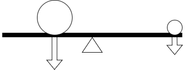
The center of mass is the point where we can place the fulcrum and keep the seesaw balanced.
Mathemathically, this is:
\[ com = \dfrac{\sum{m_i * x_i}}{\sum{m_i}} \]
We can use this to find the center of mass in both x and y dimensions. We can do this iteratively, or we can leverage numpy to vectorize our multiplications!
We should be able to test our code with some simple examples:
centerOfMass(np.array([[0, 0, 1], [0, 2, 1]]))  # [0.0, 1.0]
centerOfMass(np.array([[1, 1, 1], [1, -1, 1], [-1, 1, 1], [-1, -1, 1]]))  # [0.0, 0.0]
Next, we want to plot our data with matplotlib:
def plotObjects(objects):
    """Draw a matplotlib chart of our objects.
    We should use a scatter plot to show the objects in 2D space.
    The size of the object should be proportional to its mass.
    Finally we should annotate the center of mass with a red dot.
    To do this last part, you should be able to run:
        com = centerOfMass(objects)
        plt.scatter(com[0], com[1], s=25, c="red")

    Args:
      objects: an Nx5 matrix of (x,y,mass,vx,vy)
    """
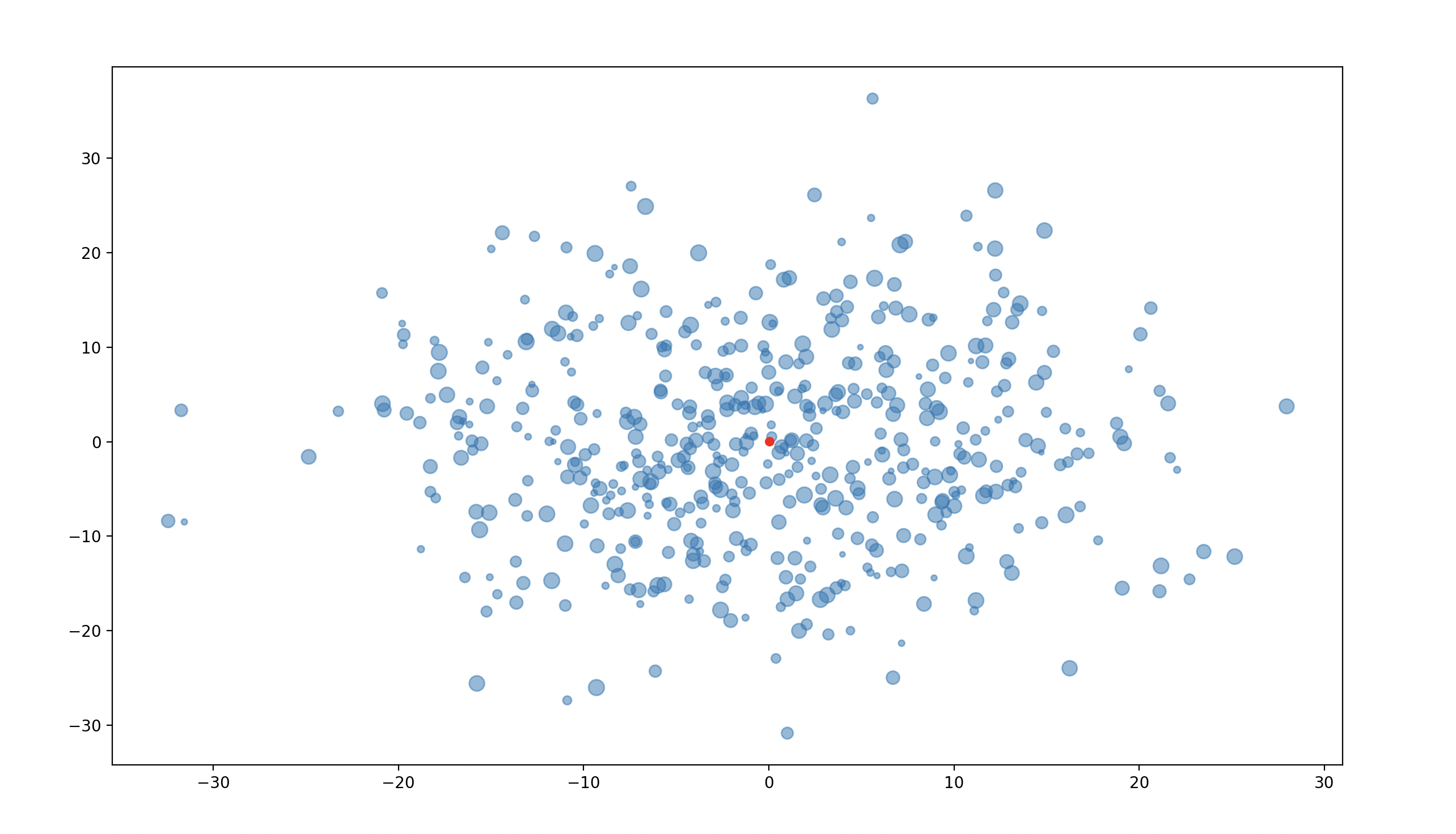
In this part, we want to plot our objects using matplotlib.
To produce a scatter plot, we can use plt.scatter.
The first argument will be the x positions, the second argument will be the y.
We can use the s positions to size the objects by mass, and alpha=0.5 makes them semi-transparent.
import matplotlib.pyplot as plt

# Create a figure
plt.figure(figsize=(14, 8))
plt.scatter(x, y, s=sizes, alpha=0.5)
Finally, we can scatter a red dot in the center of our plot using the tip in the docstrings.
When we’re done adjusting our plot, we can call plt.show() to display it.
That should look something like this:
Next, we want to calculate the distance between any 2 objects in our system:
def distance(vec1, vec2):
    """Calculate the distance between 2 points vec1 and vec2.

    Note: we only care about the first 2 fields in vec1 and vec2 corresponding to the x,y positions

    Args:
        vec1: 1x5 vector of (x,y,mass,vx,vy)
        vec2: 1x5 vector of (x,y,mass,vx,vy)
    """
In this part, we only care about the x and y coordinates. We can calculate Euclidean distance iteratively:
\[ com = \sqrt{(x_1 - x_2)^2 + (y_1-y_2)^2} \]
Or we can vectorize with numpy and use np.linalg.norm.
Again, we can rely on some standard triangles to validate our work:
distance(np.array([0, 0]), np.array([3, 4]))  # 5.0
distance(np.array([0, 0]), np.array([-3, 4]))  # 5.0
distance(np.array([0, 0]), np.array([5, 12]))  # 13.0
Next, we want to calculate the force between any 2 objects in our system using the gravitational equation from lecture.
Note the comments about G – we’re going to boost gravity’s effectiveness a little bit to produce better animations.
# NOTE: We're cheating a bit here to avoid having to deal with the true scaling differences between e.g. an individual star and a supermassive black hole.
# We're also adjusting for the fact that we'd like to deal with reasonable size masses.
G = 6.6743 * 10 ** -5


def force(m1, m2, s):
    """Calculate the force between m1 and m2 over distance s

    Args:
        m1: int/float mass
        m2: int/float mass
        s: int/float distance
    """
There are no tips or trick here, just basic equations.
Next, we want to calculate the angle between any 2 objects in our system. This is necessary for us to decompose the forces in our system into x and y dimensions so that we can sum.
def angle(vec1, vec2):
    """Determine the angle between vec1 and vec2, in 2D

    Note: we only care about the first 2 fields in vec1 and vec2 corresponding to the x,y positions

    Args:
        vec1: 1x5 vector of (x,y,mass,vx,vy)
        vec2: 1x5 vector of (x,y,mass,vx,vy)
    """
Remember sohcahtoa from grade school?
To calculate the angle between two x/y pairs, we calculate the arctangent
\[ arctan2(y_2 - y_1, x_2-x_y) \]
Again, we can validate nicely with some basic triangles:
angle(np.array([0, 0]), np.array([0, 1]))  # 1.57 - pi/2 - 90degrees
angle(np.array([0, 0]), np.array([1, 1]))  # 0.785 - pi/4 - 45degrees
angle(np.array([0, 0]), np.array([1, 0]))  # 0 - 0 - 0degrees
Next, we want to use the force and angle calculations we did previously to decompose a force into x and y components:
def forceVec(vec1, vec2):
    """Calculate the force vector between vec1 and vec2

    Args:
        vec1: 1x5 vector of (x,y,mass,vx,vy)
        vec2: 1x5 vector of (x,y,mass,vx,vy)

    The force vector should be of the form [Fx, Fy]
    """
Here are some useful numbers to validate based on a 3–4–5 triangle:
# Some nice numbers to check
# data point at 0,0 with mass 1369 and data point at 3,4 with mass 1369
# 3-4-5 triangle with hypotenuse of "length" 5
forceVec(
    np.array([0, 0, 1369]),
    np.array([3, 4, 1369]),
)

# data point at 0,0 with mass 1935 and data point at 3,4 with mass 1936
# 3-4-5 triangle with hypotenuse of "length" 10
forceVec(
    np.array([0, 0, 1935]),
    np.array([-3, -4, 1936]),
)
(3.0..., 4.0...)
(-6.0..., -8.0...)
(-6.0..., -8.0...)
Finally, we want to calculate the sum of all forces on each object in our system due to each other object in our system. Once we can do this, we have every thing we need to build the iterative simulation like we did in class.
def sumOfForces(objects):
    """Return an Nx2 array of the cumulative force acting on each object in x and y

    Args:
      objects: an Nx5 matrix of (x,y,mass,vx,vy)

    Returns:
        a (`count`, 2) array of Fx, Fy

        The return value should look like:
            [[Fx1, Fy1],
             [Fx2, Fy2],
             ...
            ]
    """
Let’s test with a set of objects in a box around the origin. Each should end up with a force pointing straight back towards the origin.
sumOfForces(np.array([[1, 1, 100], [-1, 1, 100], [1, -1, 100], [-1, -1, 100]]))
[
  [-0.22,-0.22],
  [0.22, -0.22],
  [-0.22, 0.22],
  [0.22, 0.22],
]
Putting everything above together, we can test out our data generation and calculation code by:
def main():
    # Generate a random set of objects
    objects = generateObjects(100, center=0, width=10)
    plotObjects(objects)

    # Calculate the center of mass
    com = centerOfMass(objects)
    print(f"Center of Mass: {com}")

    # Calculate the forces acting on each object
    forces = sumOfForces(objects)

    for i, obj in enumerate(objects):
        print(f"Object {i}: Position: {obj[:2]}, Mass: {obj[2]}, Forces: {forces[i]}")

if __name__ == "__main__":
    main()
Full skeleton code from the solutions is available here:
import numpy as np
import numpy as np
import matplotlib.pyplot as plt


# NOTE: We're cheating a bit here to avoid having to deal with the true scaling differences between e.g. an individual star and a supermassive black hole.
# We're also adjusting for the fact that we'd like to deal with reasonable size masses.
G = 6.6743 * 10 ** -5


def generateObjects(count, center=0, width=10):
    """Generate a `count` x 5 matrix of (x, y) coordinates corresponding to `count` number of arbitrarily placed elements

    (x,y) coordinates should be generated according to a normal distribution.
    Mass should be randomly generated integer between 10 and 100.
    (vx,vy) velocities should be 0 for this homework.

    Args:
        count (int): the number of (x, y) pairs to generate
        center (int): the center of our distribution (average if `method`=normal)
        width (int): the width of our distribution (covariance if `method`=normal)

    Returns:
        a (`count`, 5) array of positions, mass, velocities

        The return value should look like:
            [[x1, y1, mass1, vx1, vy1],
             [x2, y2, mass2, vx2, vy2],
             ...
            ]
    """


def plotObjects(objects):
    """Draw a matplotlib chart of our objects.
    We should use a scatter plot to show the objects in 2D space.
    The size of the object should be proportional to its mass.
    Finally we should annotate the center of mass with a red dot.
    To do this last part, you should be able to run:
        com = centerOfMass(objects)
        scatter(com[0], com[1], s=25, c="red")

    Args:
      objects: an Nx5 matrix of (x,y,mass,vx,vy)
    """


def distance(vec1, vec2):
    """Calculate the distance between 2 points vec1 and vec2.

    Note: we only care about the first 2 fields in vec1 and vec2 corresponding to the x,y positions

    Args:
        vec1: 1x5 vector of (x,y,mass,vx,vy)
        vec2: 1x5 vector of (x,y,mass,vx,vy)
    """


def force(m1, m2, s):
    """Calculate the force between m1 and m2 over distance s

    Args:
        m1: int/float mass
        m2: int/float mass
        s: int/float distance
    """


def angle(vec1, vec2):
    """Determine the angle between vec1 and vec2, in 2D

    Note: we only care about the first 2 fields in vec1 and vec2 corresponding to the x,y positions

    Args:
        vec1: 1x5 vector of (x,y,mass,vx,vy)
        vec2: 1x5 vector of (x,y,mass,vx,vy)
    """


def forceVec(vec1, vec2):
    """Calculate the force vector between vec1 and vec2

    Args:
        vec1: 1x5 vector of (x,y,mass,vx,vy)
        vec2: 1x5 vector of (x,y,mass,vx,vy)

    The force vector should be of the form [Fx, Fy]
    """


def sumOfForces(objects):
    """Return an Nx2 array of the cumulative force acting on each object in x and y

    Args:
      objects: an Nx5 matrix of (x,y,mass,vx,vy)

    Returns:
        a (`count`, 2) array of Fx, Fy

        The return value should look like:
            [[Fx1, Fy1],
             [Fx2, Fy2],
             ...
            ]
    """

def centerOfMass(objects):
    """Calculate the center of mass of the objects

    Args:
      objects: an Nx5 matrix of (x,y,mass,vx,vy)

    Returns:
        a single (x,y) pair corresponding to the center of mass
    """


def main():
    # Generate a random set of objects
    objects = generateObjects(500, center=0, width=100)
    plotObjects(objects)

    # Calculate the center of mass
    com = centerOfMass(objects)
    print(f"Center of Mass: {com}")

    # Calculate the forces acting on each object
    forces = sumOfForces(objects)

    # Loop through the first 10 rows and print their positions, masses, and forces
    for i, obj in enumerate(objects[:10,:]):
        print(f"Object {i}: Position: {obj[:2]}, Mass: {obj[2]}, Forces: {forces[i]}")

if __name__ == "__main__":
    main()