The goal of this note is to discuss some concepts in optimization---algorithms for choosing the weights of a neural network in order to perform well on a given objective---and discuss more neural network architecture fundamentals.
In the last note, we went through how nonlinearities allow for the construction of interesting representations of sequences. In this note, we'll introduce a few recurring elements of common neural network development.
Much ink has been spilled on the topic of optimization, the processes by which we search over the space of possible values of the parameters of our networks in order to find those that minimize the loss (which, we should keep in mind, is just a proxy for the network functioning well in practice.) In this note we'll just go over a few basic intuitions to help you think about neural architecture design. The first is what we'll roughly refer to as how well-behaved a function and its gradient are. Recall that (stochastic) gradient descent updates parameters of a network as: $$ \theta_t = \theta_{t-1} - \alpha \nabla_\theta \mathcal{L} $$ where $\mathcal{L}$ computes a loss using $\theta$ over some data, often a few examples, and $\alpha$ is an often-small scalar learning rate.
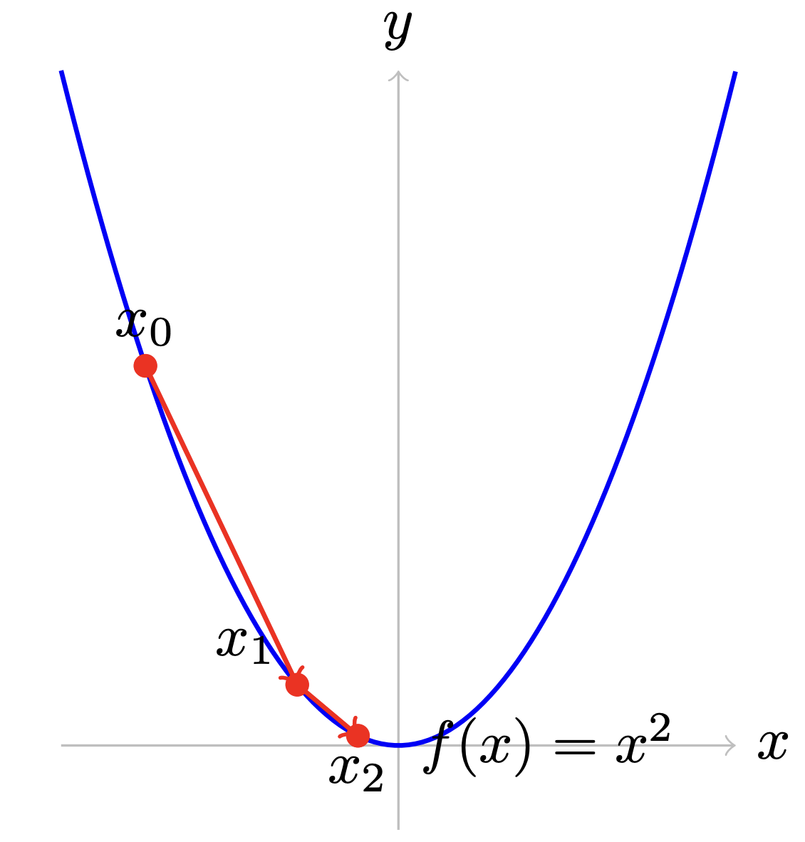
First, we'll go over thing visually, starting with a little graph showing how gradient descent takes us down a curve:
The gradient of a quadratic $x^2$ is $2x$. Gradient descent takes the gradient wherever we start ($x_0$), and moves us in the direction of the gradient a little bit: $$ \begin{align} x_1 &= x_0 - \alpha \nabla x^2\\ x_1 &= x_0 - \alpha 2x \end{align} $$ If the exponent on $x$ is larger, our gradient will be larger, like $100x$, or it could be smaller, like $0.0001x$. In either case, we could adjust our step size $\alpha$ to account for this.
Ok, now let's make things trickier, where we have a loss function which is much more sensitive to changes in one variable than another:
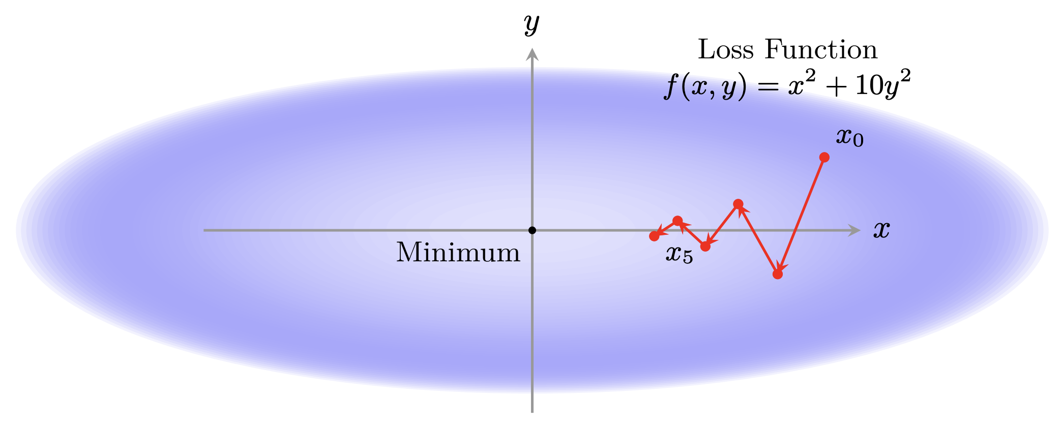
If we were to continue to stretch out the dependence on one variable compared to the other, we can see intuitively how this makes optimization difficult. Large steps for one variable are small for the other. Very large gradients can move us very far in a single step, whereas very small gradients can keep us stuck in place. As a final piece of visual intuition, take a look at two different visualizations of loss landscapes, which show in extremes how it might be difficult to search over a loss landscape using local information, taken from (Li et al., 2018).

Now let's take a linear algebraic approach to thinking about how composing even relatively nice functions can lead to some gradients that either shrink to zero or blow up towards infinity.
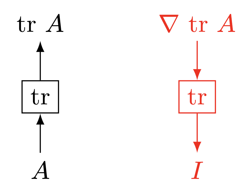
Imagine, for example, the following silly little maximization problem:1 $$ \max_{A} \text{tr}(A) $$ Here, we're taking the maximum over our matrix $A$ of the trace of $A$, that is, the sum of the elements along its diagonal. If we were to take gradients and move in the right direction locally: $$ \nabla_A A_{ij} = I $$ That is, the identity matrix, since the gradient is $0$ everywhere except the diagonal, where it's $1$. Think of this as a shallow network. Gradients are nice and well-behaved.
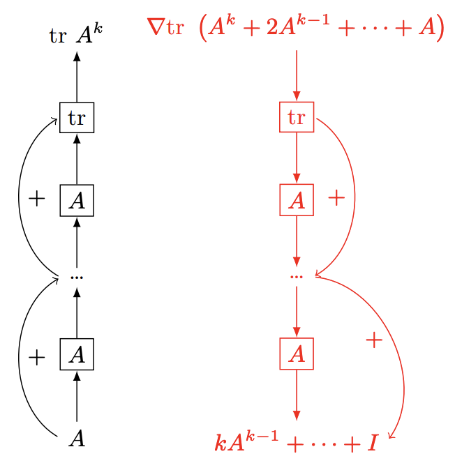
Now, what if instead our function were $f(A) = \text{tr} A^k$, and we assume $A$ is diagonalizable and symmetric?
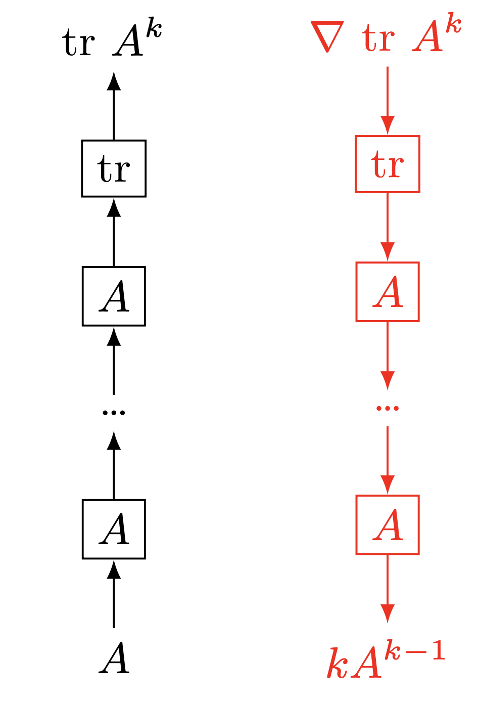
The gradient of this function looks a bit like in single variable calculus: $$ \nabla_A \text{tr}(A^k) = k\ A^{k-1} $$ As a diagonalizable, symmetric matrix, $A^{k-1}$ can be computed by taking the eigendecomposition of $A$ and taking each of the eigenvalues to the power $k-1$: $$ \begin{align} &A = P\Sigma P^{-1}\\ &A^{k-1} = P\Sigma^{k-1} P^{-1}\\ &\text{where } \Sigma^{k-1} = \text{diag}([\sigma_1^{k-1};\cdots;\sigma_{d}^{k-1}]) \end{align} $$ If all the eigenvalues $\sigma_i$ are equal to $1$, then their powers $\sigma_i^k$ are also equal to 1, so our gradient looks very nice (since $P$ is orthonormal). As we keep taking more and more powers of $A$, our gradient stays nice and close to $1$. However, let's say $\sigma_1 =1.1$, and $\sigma_2 = 0.9$. Then at large powers, $\sigma_1^k \rightarrow \infty$ and $\sigma_2^k \rightarrow 0$. Oh no! Those are not well-behaved gradients.
People have worked on improving optimization on difficult loss landscapes for many years, and separately, have found that the very large number of parameters in neural networks make optimization easier in some ways. One result of optimization research is optimizers that act like gradient descent, but are faster in practice for optimizing our networks. To give you intuition, here's a simplified version of the Adam variant of gradient descent (Kingma & Ba, 2014), which we'll go through in more detail later in the course.
$$ \begin{align} &m_t = \beta m_{t-1} + (1-\beta)\nabla_\theta \mathcal{L}& \\ &v_t = \beta v_{t-1} + (1-\beta)(\nabla_\theta \mathcal{L})^2& \text{(Elementwise squaring)}\\ & \theta_t = \theta_{t-1} - \frac{\alpha}{\color{blue}{\sqrt{v_t}+\epsilon}}\color{red}{m_t} & \text{(Adam-like simplified)} \end{align} $$$m_t$: Exponentially decaying average of past gradients (momentum).
$\sqrt{v_t}$: Exponentially decaying average of magnitude of past gradients (scaling).
Intuitively, moving in the direction of the exponentially decaying average of past gradients ($m_t$) keeps memory in the algorithm as to the direction (in parameter space) you've tended to go in recently, which turns out to be useful. The exponentially decaying average of the magnitude of the gradients ($v_t$) intuitively helps speed up movement of parameters where gradients are very small (and thus learning may be slow) and slow down movement of parameters where gradients are very large (and thus a single step may take us much too far away in parameter space). The small $\epsilon$ exists to avoid dividing by zero. The actual Adam algorithm has further adjustments, in particular to handle the start of optimization wherein one has no existing moving average.
We're about to go into a section wherein we discuss very common, useful neural network architectural components. From this mini section on optimization, I'd like you to take away the intuition that you should be thinking about how gradients are flowing through your network, whether something should be hard or easy to optimize through, whether gradients may be becoming very large or small due to decisions you're making.
As always, we're representing sequences $x_{\lt i}=x_1,\dots,x_{i-1}$ from a finite vocabulary in a vector $h_{\lt i}\in\mathbb{R}^{d}$. Consider that we have such a vector $h_{\lt i}$.
A feed-forward network (or, feed-forward layer), also sometimes called a multi-layer perceptron, is a function of the form $$ f(h) = A\sigma(Bh), $$ where $B\in\mathbb{R}^{p\times d}$, and $A\in\mathbb{R}^{q\times p}$. The input dimensionality is $d$, the hidden dimensionality is $p$, and the output dimensionality is $q$. Commonly, we choose input and output dimensionalities to be equal. As such, we could apply multiple identically-sized feed-forward layers in sequence. A feed-forward layer is often seen as a general device for adding learning capacity to a network. The inclusion of a nonlinearity at the hidden layer allows the network to compute non-linear feature combinations of whatever it was provided with, and then recombine those into the output.
Consider a neural function $f(h)$ which has the added constraint of mapping the $d$-dimensional input vector to a $d$-dimensional output (that is, the constraint is that the input and output shapes are the same.) A residual connection means we add the input of the function to the output. That is, I can add a residual connection around $f$ to define a new function $\tilde{f}$ as: $$ \tilde{f}(h) = h + f(h) $$ This addition requires the input and output shapes to be identical. Practically, residual connections are used because they improve how gradients behave in networks. My favorite intuition as for why is as follows. Consider the following neural function with parameters $A\in\mathbb{R}^{d\times d}$, and some function $f: \mathbb{R}^{d}\rightarrow \mathbb{R}^d$, that is, $f$ maps $d$-dimensional vectors to $d$-dimensional vectors, but otherwise we're not saying how. $$ \tilde{f}(h) = f(Ah) $$ So, this function first applies $A$ to $h$, and then puts it through $f$. Now let's take a loss with a function $\mathcal{L}(x) = - x^\top b$ for some specified $d$-dimensional vector $b$ vector. This loss function just wants the input to be like $b$. Ok, so let's take the gradient of this loss with respect to an element of our parameters $A_{ij}$: $$ \begin{align} \nabla_{A_{ij}} \mathcal{L}(f(Ah)) &= - \nabla_{A_{ij}} \sum_{k=1}^{d} b_k f(Ah)_k\\ &= - \nabla_{A_{ij}} \sum_{k=1}^{d} b_k f(Ah)_k\\ &= - \sum_{k=1}^{d} b_k \nabla_{A_{ij}} f(Ah)_k\\ &= - \sum_{k=1}^{d} b_k f'(Ah)_{ki} \nabla_{A_{ij}} Ah\\ &= - \sum_{k=1}^{d} b_k f'(Ah)_{ki} h_j \end{align} $$ So, let's look at these terms of the last line: $b_k f'(Ah)_{ki} h_j$. The term $b_k$ is some constant, as is $h_j$; this term in the middle, though, $f'(Ah)_{ki}$, is an element of the jacobian, the partial derivative matrix of $f$. In particular, it relates the output at index $k$ to the input at index $i$. What happens if $f'(Ah)_{ki}$ is zero? Then the gradient is zero, and no signal from our loss makes its way back to $A_{ij}$, so we learn nothing. What if $f'$ is not quite zero, but something small, like .25, and then we apply many such $f$? Then when we take the products of the gradients, we get $.25^n\approx0$. A residual connection avoids this by ensuring there's always a simple gradient connection: $$ \begin{align} \nabla_{A_{ij}} \mathcal{L}(\tilde{f}(Ah)) &= \mathcal{L}(f(Ah) + Ah)\\ &= - \nabla_{A_{ij}} \sum_{k=1}^{d} b_k \left(f(Ah)_k + Ah_k\right)\\ &= - \sum_{k=1}^{d} b_k \left( \nabla_{A_{ij}} f(Ah)_k + \nabla_{A_{ij}} (Ah)_k\right)\\ &= - \sum_{k=1}^{d} b_k \left( f'(Ah)_{ki} h_j + \nabla_{A_{ij}} (Ah)_k\right)\\ &= - \sum_{k=1}^{d} b_k \left( f'(Ah)_{ki} h_j + h_k\nabla_{A_{ij}}(A)\right)\\ &= \color{blue}{-\sum_{k=1}^{d} \left(b_k f'(Ah)_{ki} h_j\right)} \color{red}{- b_ih_j} \end{align} $$
Blue term: Gradient through the possibly complicated, poorly behaving function $f$.
Red term: Nice simple gradient that skips $f$.
So, the gradient terms for our $A_{ij}$ are the sum of the original term (with $f'(Ah)_{ij}$ in the sum,) and a new term $b_ih_j$, which is pulled out of the sum over $k$. This is because the gradient of $A_{ij}$ is only non-zero at index $i=k$ in the sum, and for index $j$ into the vector $h$.
Gating helps control the flow of effects through a network. Imagine I have some representation $h\in\mathbb{R}^{d}$ and there's some function that modifies $h$ as $$ h \leftarrow h + v $$ for some vector $v$, where the left arrow $\leftarrow$ means assignment of a new value to $h$ (which we're using here for ease of notation.) This says that no matter the value of $h$, add $v$. But what if we should only add $v$ depending on some properties of $h$? Here's a simple gate: $$ h \leftarrow h + \sigma(h^\top v) v $$ Now, we're taking a similarity between $h$ and $v$, and then normalizing it to $(0,1)$ through the sigmoid function. That multiplication by a scalar between $0$ and $1$ is the gating. That gate is multiplied by $v$, so this says we only add $v$ to the extent it's already similar to $h$.
This is a scalar gate; the same scalar between $0$ and $1$ is applied to all $d$ dimensions of the addition of $h$ to $v$. We can also have elementwise gates; here's one: $$ h \leftarrow h + \sigma(h)\odot v $$ Here, we're taking $h$, and for each element, we're normalizing it to between $0$ and $1$. That gate $\sigma(h)$, which is itself a vector in $\mathbb{R}^{d}$, is then elementwise multiplied with $v$. So, this update is saying that each element $h_i$ has the corresponding $v_i$ added to it more if $h_i$ is very negative, and less if $h_i$ is very positive.
Gates are used in many architectures to build in mechanisms for determining when to write, read, or forget data. In the examples above, one could see the gates we constructed as reading gates, determining when to read from $v$. Here's an example that also decides what of $h$ to forget (or, remember.) $$ h \leftarrow \sigma(-h)\odot h + \sigma(v)\odot v $$ This gated function reads from each element $v_i$ to the extent that it's large and positive, and remembers each element $h_i$ to the extent that it's large and negative.