Lec 1: Text Representation and Language Modeling

Class Topics

How do we build computer programs that learn from human language text? How do we build computer programs that learn to understand and generate human language text? This course provides an introduction to Natural Language Processing (NLP), the field dedicated to these questions.

Here are a few goals of the course:

• Teach you the core techniques and algorithms used in the field to build NLP systems.
• Teach you about the process of developing---building, evaluating, improving---NLP systems.
• Help you develop intuitions about how to tackle new NLP-related problems.
• Give some flavor of cutting-edge NLP techniques and how they are changing today.

Inspiration

What can you learn from observing text?

Two core concepts we’ll return to again and again in this course are how to represent text, and how to generate outputs that relate to that text. As we’ll see, the answers to these two questions will be deeply related.

Keep in mind that there is an internet of text to learn from, and more. Imagine how much knowledge is stored, how many skills, how many facts, but also how many social biases, how much hatred.

Representing text as strings of characters

So, how do we represent text? Here's an example.

Uncle Iroh is a wise man.

This is a string of unicode/ascii characters. This is a representation, and is good for comparisons like $$ \texttt{Uncle Iroh is a wise man.} \neq \texttt{Zuko is a wise man.} $$ What if we want to ask which of two pairs of strings is more similar (here written as the function sim)?

• sim(Uncle Iroh is a wise man, Uncle Iroh is a smart man)
• sim(Uncle Iroh is a wise man, Uncle Iron is a worse man)

A string of ascii characters can be compared via string edit distance, but here, string edit distance doesn't correspond to intuitive similarity. The problem is that “worse” shares more characters with “wise” than does “smart”, but “wise” and “smart” are more similar. One might ask — how do we know those are “words” — all we know is that they’re different strings of characters! This is a good question which we’ll address in-depth in future lectures, but for now, we’ll incorrectly but usefully assume that characters separated by spaces give a good-enough approximation of words.

Representing ‘words’

So, how do we represent words?

smart
wise
worse

One idea is to assume that there’s a finite vocabulary of words, and each word gets a unique arbitrary identifier. So, for example, we give some arbitrary order to our words, and let the index in the order represent the word:

[
    “smart”,		# 0
    “wise”,		# 1
    “worse”,		# 2
    …
]

In this representation, “smart” is just the 0th word, dissociated from its spelling.

We can compare it to another word “smart”, see that they’re both 0th, and say they’re the same, or we can compare it to a different word, like “wise,” see that $0 \neq 1$, and say they’re different. It is common to represent this in a so-called one-hot vector encoding; a vector of the size of our vocabulary, with a 1 at the correct index for the word, and zeros everywhere else:

• smart: $[1,0,\dots]$
• wise: $[0,1,0,\dots]$
• pizza: $[0,\dots,1,0,\dots]$

Comparison can be achieved here via, e.g., $L_1$ distance:

• $\|v_{\text{smart}} - v_{\text{wise}}\|_1 = |1-0| + |0-1| + |0-0| + \dots = 2$
• $\|v_{\text{smart}} - v_{\text{smart}}\|_1 = |1-1| + |0-0| + \dots = 0$

When words are represented as vectors, the vectors are often called word embeddings. But these embeddings are not so helpful! Intuitively, there are components of meaning that words can share or not share, and we need to compare those. One idea is to hand-craft components of meaning and label each word in your finite vocabulary with the value of that component.

Here are some potential components:

• related to intelligence
• related to wisdom
• related to comparison

If we represent our words along these three components, we get

• smart:
  • related to intelligence: yes
  • related to wisdom: no
  • related to comparison: no
• Or
• smart: $[1, 0, 0]$

And likewise,

• wise: $[1,1, 0]$
• worse: $[0, 0, 1]$

Now we have

• $\|v_{\text{smart}} - v_{\text{wise}}\|_1 = |1-1| + |0-1| + |0-0| = 1$
• $\|v_{\text{smart}} - v_{\text{worse}}\|_1 = |1-0| + |0-0| + |0-1| = 2$

Correctly indicating that smart is more similar to wise than it is to worse!

Pack it up; let’s go home. We’ve solved it. All we have to do now is exhaustively enumerate every distinction in word meaning, and annotate every word for it. What are the problems here?

• You’re never right about what the distinctions should be or how to annotate them. Language is rich and varied and it defies manual enumeration of said variation.
• This is too much work and too vague work to properly annotate the distinctions for everything.

Let’s go back to the beginning of the lecture, where we demonstrated how much we can learn from filling in—predicting— missing text. As we’ve stated, representing text and predicting text will be in some sense each others’ solutions.

Representing and generating text jointly

The basic idea of learning representations by prediction is that prediction problems are hard; you have to understand quite a bit about the text in order to do a good job of predicting parts of it that you can’t see. There are a few components we’ll need to make this concrete.

Let’s take two texts:

• Uncle Iroh was so smart
• Uncle Iroh was so wise

And turn them into prediction problems:

• Input: Uncle Iroh was so
• Output: smart

• Input: Uncle Iroh was so
• Output: wise

Knowing to predict either “smart” or “wise” means

1. we know what kind of words can follow “was so” (roughly, adjectives).
2. We know about Uncle Iroh enough to know what kinds of things he’d be called.
3. We know that wise and smart are similar.

When we make our prediction, we have to accept that many words could appear after Uncle Iroh was so. Our prediction should be probabilistic, quantifying uncertainty about the next word.

Language Modeling

Language modeling is the task of determining a probability distribution over strings.

Let $V$ be a finite vocabulary, and $w \in V$. A string is $(w_1, \dots, w_k) \in V^*$. We write a probability distribution over $V^*$ as $$ P(w_1, \dots, w_k) $$ We can decompose this probability via the chain rule of probability as $$ P(w_1, \dots, w_k) = \prod_{i=1}^{k} p(w_i | w_{\lt i}) $$ For our example, we could for example write:

• $P(\text{smart} | \text{Uncle Iroh was so}) = 0.5$
• $P(\text{wise} | \text{Uncle Iroh was so}) = 0.5$

A Word-Based Language Model

Our goal is to build a language model that uses word representations, and in doing so, allows us to learn those word representations.

Let’s start with a simple word representations we haven’t considered yet: randomly sampling a vector in some dimensionality, and using that as the representation of a word.

• $v_{\text{smart}} \sim U[-0.001, 0.001]^d = [0.0004, -0.0003, \dots]^T$
• $v_{\text{wise}} \sim U[-0.001, 0.001]^d = [-0.0001, 0.0009, \dots]^T$

With these representations of words, we can come to a simple representation of prefixes where we just average the embeddings of all words so far: $$ h(w_{\lt i}) = \frac{1}{i} \sum_{j=1}^{i-1} v_{w_j} $$ This is an odd representation of the text, but for now we’ll go for it. The main concern is that it doesn’t distinguish between different orderings of the same word, but again, for now let’s ignore that problem.

We can form a distribution over the next word by computing vector similarities between each word and the representation of the prefix, and then normalizing the similarities by the total sum of similarities to all words. $$ P(w_i \mid w_{\lt i}) = \frac{ \exp(v_{w_i}^T h(w_{\lt i}))}{\sum_{j \in V} \exp(v_{w_j}^T h(w_{\lt i}))} $$ This is a probability distribution because (1) it sums to one, and (2) all terms are non-negative (because of the exponentiation.) We now have a language model! It averages together all word embeddings for the prefix, and then predicts the next word by comparing that average to the embedding of each word in the vocabulary. The more similar each word’s embedding is to the average so far, the higher-probability it will be.

Learning from text with a language model

The general process of learning will be to

1. specify a single summary of how bad a job we’re doing at the prediction process with our language model, and
2. tweak the representations of our model in order to do slightly less badly. Then repeat.

Imagine I could grab a random text, say from the internet, as many times as I wanted. I’d like the average probability I assign to any such text to be high. We write this as $$ \mathbb{E}_{(w_1,\dots,w_k) \sim D} \left[ P(w_1,\dots,w_k)\right]. $$ We’d like to maximize this overall prediction quality. But for various reasons including numerical stability, we’ll pick a monotonic function — the logarithm — and work with the log-probability instead. We’ll also add a negative sign and minimize instead of maximizing, because of machine learning convention. So, our learning objective is: $$ \text{Minimize} \quad \mathbb{E}_{(w_1,\dots,w_k) \sim D} \left[ -\log P(w_1,\dots,w_k)\right]. $$ Now, what are we minimizing this over? That is, what stuff are we changing in order to perform this minimization? The word embeddings: $$ \min_{v_w, w \in V} \mathbb{E}_{(w_1,\dots,w_k) \sim D} \left[ -\log P(w_1,\dots,w_k)\right]. $$

Gradient-based learning from text

The last component is, how do we do the tweaking of word embeddings to make them better for this prediction problem? The answer is by taking gradients. Intuitively, a gradient tells you the best way to (locally, slightly) tweak a continuous value in order to minimize a function value.

So, the process is: $$ v_w \leftarrow v_w - \epsilon \cdot \nabla_{v_w} L $$ What’s that gradient look like? $$ \begin{align*} \nabla_{v_w} L &= - \nabla_{v_{w_i}} \log P(w_i \mid w_{\lt i}) \\ &= - \nabla_{v_{w_i}} \left( v_{w_i}^T h(w_{\lt i}) - \log \sum_{j \in V} \exp(v_{w_j}^T h(w_{\lt i})) \right) \\ &= - h(w_{\lt i}) + \frac{1}{\sum_{j \in V} \exp(v_{w_j}^T h(w_{\lt i}))} \sum_{j \in V} \exp(v_{w_j}^T h(w_{\lt i})) \nabla_{v_{w_i}} (v_{w_j}^T h(w_{\lt i})) \end{align*} $$ This last gradient, $\nabla_{v_{w_i}} (v_{w_j}^T h(w_{\lt i}))$, depends on whether our target word $w_i$ shows up in the context $w_{\lt i}$. (Has this word showed up already in the prefix?) This is sort of annoying but doesn’t change anything fundamentally. Let’s take the simpler case for now, where it doesn’t show up in the prefix so far: In this case, the gradient with respect to the target word embedding $v_{w_i}$ is: $$ \begin{align*} \nabla_{v_{w_i}} L &= - h(w_{\lt i}) + \frac{1}{\sum_{j \in V} \exp(v_{w_j}^T h(w_{\lt i}))} \exp(v_{w_i}^T h(w_{\lt i})) h(w_{\lt i}) \\ &= - h(w_{\lt i}) + P(w_i \mid w_{\lt i}) h(w_{\lt i}) \\ &= -(1-P(w_i \mid w_{\lt i})) h(w_{\lt i}) \end{align*} $$ this is just saying, make my $v_{w_i}$ more like its context $h(w_{\lt i})$, with a weight proportional to how bad a job I was doing at predicting $w_i$! The less weight I had put on $w_i$ before, the greater the size of the update.

What does this end up doing?

Training a model like this leads to a vector per word in our vocabulary that has fascinating structure.

We trained a 100-dimensional model of this form on linux-related text data, roughly 1B tokens' worth. Our context window was the preceding 10 words before each predicted context word.¹ Once trained, we took some query words, like linux, took their embedding $e_{\text{linux}}$, and then found their nearest neighbors: $$ \text{nearest}(\text{linux}) = \arg\max_{w\in\mathcal{V}} v_\text{linux}^\top w. $$ Here are some nearest neighbors:

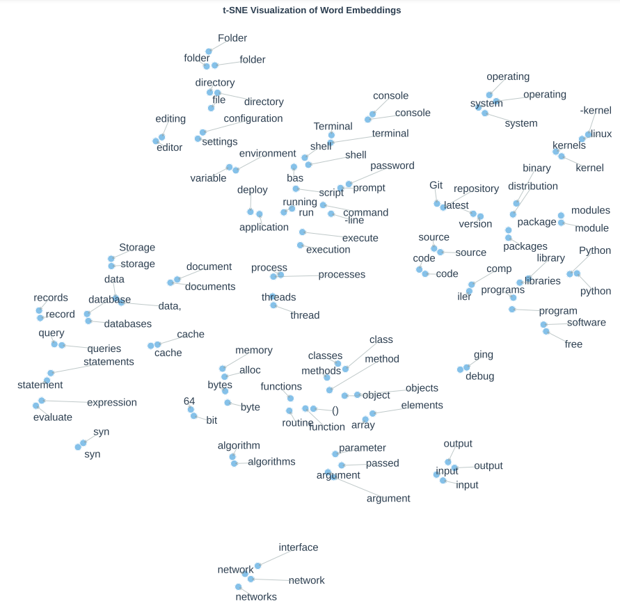
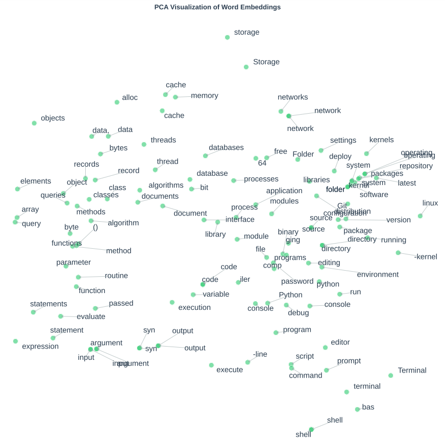
Note how we've unsupervisedly learned, from the text data, that some words are similar to each other. There are some visualization methods we can use to peek a bit more at the structure learned, for example, principal components analysis, which visualizes linear structure, in Figure 1. Another method for visualization is t-SNE, which is a murky, non-linear visualization that can lie to you a bit in seemingly suggesting structure that isn't there, but is yet fun to look at if you're careful (Figure 2.) I've made these full page figures (below) so you can best see them.

Why care about these word embeddings?

Modern language models do much more powerful things than showing similarities between words. But the framework we've introduced here---(1) build a representation for a prefix of text, (2) map that representation into a distribution over the vocabulary, (3) learn that distribution from a large body of text---is the foundation of modern natural language processing system building. The only two differences, in a sense, are the function we use to compute the representation of the prefix, and the distribution of text we train on.

…