Lec 3: Neural Networks and Sequence Representation

COMS 4705: Natural Language Processing
Columbia University · John Hewitt

The goal of this note is to give an overview of basic neural network components and considerations when modeling text.

Consider the text modeling problem we've considered so far. We have sequences $x_1, \dots, x_n$ over a finite vocabulary $\mathcal{V}$. We want to define probability distributions:

This $p(\cdot \mid x_{\lt i})$ notation denotes a $|\mathcal{V}|$-dimensional probability distribution, that is, a distribution over the vocabulary representing the probability of each word in the context of the prefix $x_{\lt i}$. We model this by (1) representing the prefix $x_{\lt i}$, and (2) projecting that representation to the space of the vocabulary, and (3) normalizing to a probability distribution using the softmax function. That is,

where $h_{\lt i} \in \mathbb{R}^d$ for some fixed dimensionality $d$, and $U$, often called the "unembedding" or "softmax" matrix, is of shape $\mathbb{R}^{|\mathcal{V}| \times d}$. Holding this form constant, the question becomes, how do we represent the prefix $h_{\lt i}$?

Representing Text through Vector Averages

One simple way to represent a prefix of text is to embed each token in $\mathbb{R}^d$, and then average the embeddings. To represent this embedding, we often use a matrix $E \in \mathbb{R}^{d \times |\mathcal{V}|}$, and consider each word $x_i$ to be a vector in $\mathbb{R}^{|\mathcal{V}|}$, so that

is a vector in $\mathbb{R}^d$. Representing our prefix $x_{\lt i}$ as an average of all word embeddings is thus

So, what's good and what's bad about this way of representing text? In the good column, it's (1) pretty cheap, and (2) parallelizable. We'll talk more about paralellization later, but for now, consider how I can compute $h_{\lt 4}$ at the same time as I compute $h_{\lt 3}$ if I want; representations of later prefixes don't depend on representations of earlier prefixes.

There's one glaring issue here, though. This representation doesn't depend on the order of the words. That is, if I took the prefix "Uncle Iroh ran to Zuko" and the prefix "Zuko ran to Uncle Iroh", these would receive the same representation, despite certainly having different meanings.

Can we just add in the positions?

Let's think through how we can incorporate the information of the positions of words into our representation of the prefix $x_{\lt i}$. Consider the following simple proposal. If we have a maximum sequence length $m$, then really, each position is an element from a finite vocabulary of positions $1, \dots m$. Just like we embedded elements from our finite vocabulary $\mathcal{V}$, we can embed elements from our positions! Let $p_1, \dots, p_m$ be vector embeddings of our positions $1, \dots, m$, each a vector in $\mathbb{R}^d$. (As always, imagine that they're randomly initialized.)

Now that we have position embeddings, let's try just adding in each position embedding to the corresponding word embedding in our average:

Is this better than our previous position-independent average? Alas, no. In fact, this representation is also invariant to the ordering of the words in the prefix. Oops! Let's see why:

What's happened here is that due to additivity, there's nothing tying each position (embedding) to each word (embedding). It all gets added together, so the fact that word $x_j$ appeared "with" position embedding $p_j$ is lost in the commutativity of addition. We need to combine the information of the word and its position in another way before we add things together and that pairing information is lost.

How about we combine with a linear transformation? Let $A \in \mathbb{R}^{d \times d}$, a linear transformation. (Again, imagine the entries in this matrix are just randomly sampled from small noise, like $\mathcal{N}(0, \epsilon)$.) Now consider:

Non-linearity for building representations

Ok, that didn't work either. The linear transformation distributes, and then we're left with exactly the same additivity problem we had before. We have to non-linearly combine our word and position information. Non-linearity is powerful in that it binds variables together; it can compute new representations of objects that don't decompose into independent contributions from each element.

What does a nonlinearity mean? Often we use this term to refer to operations that compute a (non-linear) elementwise transformation of a vector. By "elementwise" we mean that each dimension of the vector has a function performed on it independently of the values of all the other dimensions. Some famous examples are $\max(0,x)$ and the sigmoid, $\frac{e^x}{1+e^x}$. When we don't care exactly which nonlinearity is being used, we often just call the function $\sigma$. so, $\sigma(v)$ for some vector $v$ computes the scalar function $\sigma$ on each element on $v$.

Let's use some nonlinearity $\sigma$ to bind the information in each word to its position before we average them together:

Note how I can't decompose $\sigma(Ex_j + p_j)$ into $\sigma(Ex_j) + \sigma(p_j)$. (Why?) So, if I have a word $x \in \mathcal{V}$, it now matters whether it shows up at position $j$, resulting in representation $\sigma(Ex + p_j)$, compared to position $k$, resulting in representation $\sigma(E_x + p_k)$.

Batched representations

At this point, it's time to change up our mental model of representations of a sequence from what we've thought about so far—a sequence of $\mathbb{R}^d$ vectors, one for each token index—to a format more consistent with how we'll think about this for the rest of the semester. These will be mathematically equivalent, but relevant for perspectives on parallelization on a GPU, and getting the tensor operations right.

Let's take our sequence $x_1,\dots,x_T$, a sequence of $T$ tokens. We've thought of this corresponding to a sequence of representations $h_{\lt 1},\dots,h_{\lt T}$, where $h_{\lt i}\in\mathbb{R}^{d}$. Now we'll instead think of a single matrix composed of all of them.

Even worse, we may consider having $B$ sequences, a batch thereof, so maybe we have $x^{(i)}_{1},\dots, x^{(i)}_T$ for $i\in\{1,\dots,B\}$. In this case, we add another axis to our tensor (usually at the beginning), letting:

What if some of the $B$ sequences have different lengths? We'll get into this later but we usually just pad sequences to a specific length, or construct the batches so that this isn't true.

Why bother with this? Well, all of your pytorch code will look like this; we compute on batches for efficiency on the GPU (again which we'll get into later.) We do big matrix multiplies, like the following. Let $H\in\mathbb{R}^{B\times T \times d}$ be a batch of representations as we've stated above. Consider a linear transformation $W\in\mathbb{R}^{d\times d}$ that we want to apply. Then we can compute:

Well, $H$ is a tensor and not a matrix, so maybe it's not immediately obvious. But the shape $H$ is (B, T, d) and the shape of $W$ is (d, d) so it's not too ambiguous—this tensor-matrix multiply is like $B$ independent matrix multiplies between a matrix in $\mathbb{R}^{T\times d}$ and a matrix in $\mathbb{R}^{d\times d}$. So, you can think of this as linearly transforming all the representations of all the prefixes of all the sequences in the batch, all with the same linear transformation. Cool!

Information flow and simple attention

A simple average is just not that interesting, even if we've thought through the nonlinearities necessary to bind sources of information like word identity and position.

One strong intuition in representation learning is that the representation of each unit (here, token) should pull in different kinds of information from different places in the rest of the input. Right now, every word looks, equally to all previous words. We'll now introduce the concept of attention, in which each word dynamically determines which previous tokens to draw in information from. Intuitively, we're just replacing our simple average with a weighted average.

For now, I'll show both the single-vector and the batched form. First, the single-vector form:

Ok, so $\alpha_{ij}\in\mathbb{R}$ is our attention weight, which we haven't yet said how we'll define. But it's nonnegative, and the sum over all the sequence so far of the attention weights is $1$. Seems like a probability distribution over the sequence! But it's better thought of as a weight with which word $i$ wants word $j$ in its representation.

Here's a reasonable way of computing the weights: just compute the similarities between $x_i$ and each $x_j$. If $x_i$ is like $x_j$, then it should pull in some information from $x_j$. So:

Nice enough; now, our prefix representations have words looking back into the sequence to find similar-ish words and pulling in information from them. Not perfect, but better!

Now the block representations as promised. Let $X\in\mathbb{R}^{T\times |\mathcal{V}|}$ be our input sequence of tokens. We compute the embedded sequence through $H=XE^\top$, where $E\in\mathbb{R}^{d\times |\mathcal{V}|}$ is our embedding matrix.¹ Then to compute our $\alpha$, we compute all pairs of similarities through:

The first thing you want to convince yourself of is that $XX^\top$ computes a matrix $e$ such that $e_{ij} = x_{i}^\top x_j$. This is the way to enlightenment. The softmax being taken over the second axis is another difficult thing to visualize. Intuitively, it means if we sum over the second axis, the resulting vector (in $T$ dimensions) is one in each column. Put another way, the first axis represents the queries (we don't sum over the query axis!) The second axis represents the keys (we do sum over this axis.) The figure below visualizes this.

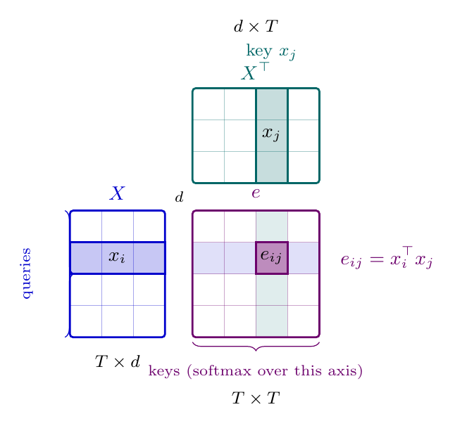
That $e$ is $T\times T$: every query is dotted with every key. In the per-position equations above, the sums ran only up to $i-1$. Here those limits have to be enforced explicitly, because nothing in the matrix multiply stops index $i$ from looking at $j\ge i$ (or $j>i$).

When performing language modeling like we've seen in this course (often called autoregressive modeling), we predict a word given all words so far:

where $f$ is function to map a sequence to a vector in $\mathbb{R}^{|\mathcal{V}|}$.

One crucial aspect of this process is that we can't look at the future when predicting it—otherwise the problem becomes trivial.

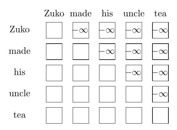
In this matrix form, there's nothing explicit in the self-attention weight $\alpha$ that says not to look at indices $j>i$ when representing token $i$. In practice, we enforce this constraint simply adding a large negative constant to the input to the softmax (or equivalently, setting $\alpha_{ij}=0$ where $j>i$.)²

In a diagram, it looks like the figure below. We'll write that additive logit mask as $M$, with $M_{ij}=0$ if $j\le i$ and $M_{ij}=-\infty$ (or a large negative constant) otherwise:

Once you've done that, you're ready to see how we batch-compute the actual weighted average. Take a look at this:

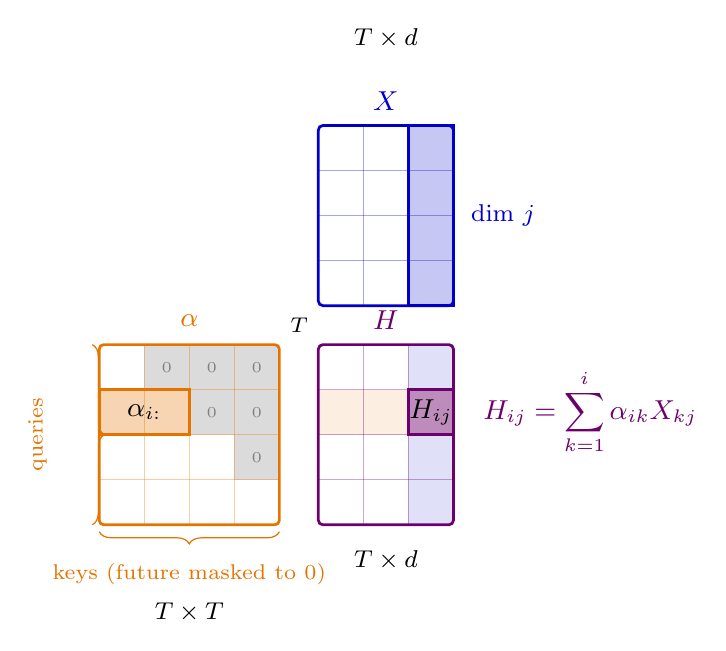
So, $H\in\mathbb{R}^{T\times d}$ since $\alpha\in\mathbb{R}^{T\times T}$ and $X\in\mathbb{R}^{T\times d}$. I claim that $H_{i}$ is exactly the weighted sum $h_{\lt i}$ that we defined above. We can see this by, e.g., writing out:

So this is dimension $j$ of what I'm claiming is the $h_{\lt i}$ vector. What is it? Well $\alpha_{ik}$ is the weight (in $\alpha$) that vector index $i$ attends to vector index $k$. That's the weight in our weighted sum, and because of the mask it is zero for $k>i$, so the sum is only over the prefix. And that weight is multiplied with what? The dimension $j$ of the vector at index $k$. So, each dot product computed in $\alpha X$ computes the weighted sum for a single dimension in each of the output vectors. Cool! The figure below visualizes this.

To complete this, imagine $X$ had an additional batch dimension, $X\in\mathbb{R}^{B\times T\times D}$. All of this would be the same, parallelized across the batches $B$. The matrix multiply semantics would be as we've presented them here.