
This exam has nine questions. The first four are intended to have very short answers. All questions vary in difficulty and topic, so I recommend searching around for those you're more familiar with first. I don't expect many people will achieve a perfect score, so keep that in mind if you're struggling. I recommend putting some thoughts down for each question at least, as we will be giving partial credit. Write your UNI and name on the TOP RIGHT of every page.
Given a distribution $p_\theta$ over strings over a vocabulary $\mathcal{V}$ that includes an EOS token, describe the condition under which the greedy decoding generation process terminates. (The answer should be a single sentence.)
The greedy decoding process terminates when the EOS token is the most likely token under the model’s conditional distribution at the current step.
I have two possible prompts for asking for the location of Columbia University.
Where is Columbia University located? Columbia University is located inThere are likely more examples in the training set that are of the format "Columbia University is located in New York" than "Where is Columbia University located? New York". The question/answer formatting of information is less common.
Consider performing DPO on a preference dataset $$ \begin{align} \{(x, y_c, y_r)_i\}_{i=1}^{k} \end{align} $$ where preferences come from a model $\phi(\hat{y},x)$ compared to running Simple Reward Learning with a rollout count of $2$ on $\{x\}_{i=1}^{k}$ (the same $x$ question set), where preferences also come from $\phi(\hat{y}, x)$.
What is the fundamental difference between these two strategies? The answer should be a single sentence.
DPO directly optimizes the policy using a fixed dataset of preference pairs $(y_c, y_r)$, giving a static distribution of responses, whereas SRL generates new outputs from the current model at each training step and uses their rewards to update the policy dynamically.
I have roughly 1000 examples of problems I'm trying to solve. I'm testing providing them as few-shot examples to my language model. At first, the model's performance improves with more examples, but then my python script crashes when I use 100 or more.
What went wrong, and what should I do? The answer should be roughly two sentences.
The script crashes because the model's input exceeds its context window when too many few-shot examples are included. To fix this, you can reduce the number of examples per prompt, use a model with a larger context window or memory mechanism, or alternatively fine-tune the model on your examples to avoid exceeding the context limit.
The feed-forward layers in Transformers often have larger hidden dimensionality than the ambient dimensionality $d$ of the model. Here we'll see one reason why.
Part a. Consider the first step of a feed-forward layer---a linear transformation. Let $A\in\mathbb{R}^{d\times d}$, and an input $X\in\mathbb{R}^{d\times b}$, where $b$ is a batch size. Then the linear transformation is $$ \begin{align} AX \end{align} $$ Assuming 32-bit floating-point numbers, what are the number of floating-point operations, and the number of byte accesses of this function? Write these and the arithmetic intensity.
Part b. Now compute the same for $C\in\mathbb{R}^{5d\times d}$, and as before, $X\in\mathbb{R}^{d\times b}$. The layer is thus $$ \begin{align} CX \end{align} $$ As before, 32-bit floating-point numbers, what are the number of floating-point operations, and the number of byte accesses of this function? Write these and the arithmetic intensity.
Part a. Assume 32-bit floats (4 bytes).
$$ \text{FLOPs} = d^2 b \quad (\text{plus lower-order terms}) $$ $$ \text{Bytes (no write)} = 4(d^2 + db) \quad\text{(read $A$ and $X$)} $$ $$ \text{Bytes (with write)} = 4(d^2 + db + db) \quad\text{(also write $AX$)} $$ $$ \text{Arithmetic intensity (no write)} = \frac{d^2 b}{4(d^2 + db)}, \qquad \text{with write: } \frac{d^2 b}{4(d^2 + 2db)} $$
Grading note: Full credit is given whether write accesses are included or not.
Part b. Assume 32-bit floats (4 bytes). $$ \text{FLOPs} = 5d^2 b \quad (\text{plus lower-order terms}) $$ $$ \text{Bytes (no write)} = 4(5d^2 + db) \quad\text{(read $C$ and $X$)} $$ $$ \text{Bytes (with write)} = 4(5d^2 + db + 5db) \quad\text{(also write $CX$)} $$ $$ \text{Arithmetic intensity (no write)} = \frac{5d^2 b}{4(5d^2 + db)}, \qquad \text{with write: } \frac{5d^2 b}{4(5d^2 + 6db)} $$
Grading note: Full credit is given whether write accesses are included or not.
Recall Low-rank Adaptation, in which we finetune a neural network by learning only a low-rank update to each matrix, like: $$ \begin{align} \tilde{A} \leftarrow A + uv^\top \end{align} $$ for $A\in\mathbb{R}^{m\times n}$, and $u,v\in\mathbb{R}^{d}$.
Let $\|u\|=\|v\|=1$. Now, consider a vector $z$, with $\|z\|=1$. Show that $\|Az - \tilde{A}z\|\leq 1$.
$$Az - \tilde{A}z = Az - (A + uv^\top)z =Az - Az - uv^\topz = -uv^\topz$$
$$\|Az - \tilde{A}z \| = \|-uv^\topz\|
= \|uv^\topz\|
= \|u\| v^\topz
= v^\topz$$
Since both $v$ and $z$ are unit-norm, then $v \cdot z \leq 1.$
Imagine you are given a large corpus of web text, $\mathcal{D} = \{D_1, D_2, ..., D_N\}$ where each document $D_i = w_{1}...w_{T_{D_i}}, w_j \in \mathcal{V}$. You want to use this data to create a pretraining corpus, so you will develop a model-based quality filter. To train the filter, you label texts from Wikipedia, Books, and similar sources as high-quality documents. You label texts randomly sampled from CommonCrawl as low-quality documents (This is a replicated setup for the PALM quality filter, and the plot below shows real outputs of the filter.). After fitting the model, you look at the distribution of predictions on the original high-quality sources, original low-quality sources, and your data pool, $\mathcal{D}$. But uh oh, you poorly labeled your data files and don't know which corpus is which. You do know that the distributions of model outputs on the three data sets looks like the following (the figure below): 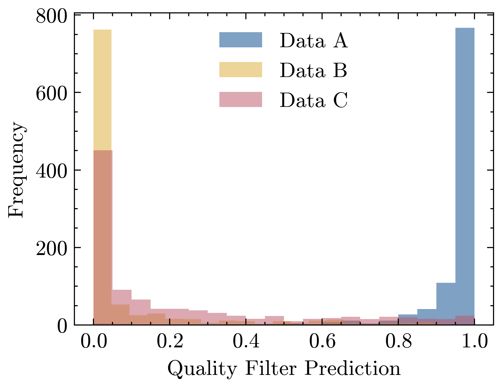
What data sets do "Data A", "Data B", and "Data C" likely represent? Why do you think so based on the distributions?
Data A represents the original high-quality data, Data B represents the original low-quality data, and Data C represents samples from our data pool. Because the classifier was trained on the original high and low-quality sources, we expect these distributions to be highly concentrated around 0 and 1 respectively. Importantly, this does not necessarily mean that the original low quality sources are all low quality; as we discussed in lecture, CommonCrawl may contain some high quality documents, but because we use them as the negative class in training the classifier, we don't expect the filter to label any of these documents as high quality. While Data C is similarly a random sample of web text, it was not explicitly included in training, and so we expect to see a concentration around 0 but more distributed predictions from 0 to 1.
Correctly assigning Data A, B, and C was worth a total of 1 point. Even if solutions did not explicitly use the original high/low quality sources and data pool, we gave credit for assignments we felt were sufficiently close to these datasets. The explanations for Data A and Data B were worth 1 point total. Explanations generally received credit if they discussed that Data A represents primarily high quality predictions and Data B represents primarily low quality predictions. The explanation for Data C was worth 2 points. Full credit was only received if the solution sufficiently distinguished Data B and Data C. As both are really random web texts and contain a mix of document quality, the primary difference is that the original low-quality sources were included in training. Strictly explaining that Data C contains a mix of document quality or is a more uniform/variable distribution is not completely sufficient to distinguish Data B and C, so these solutions received a small penalty.
Consider self-attention, in which we have an input set $h^{(\ell)}_1,\dots,h^{(\ell)}_n$, and we define our output set as $$ \begin{align} &h^{(\ell+1)}_i = \sum_{j=1}^{n} \alpha_{ij} W_V h^{(\ell)}_j\\ &\alpha_{ij} = \frac{\exp((W_Q h^{(\ell)}_i)^\top (W_K h^{(\ell)}_j))}{\sum_{j'=1}^{n} \exp((W_Q h^{(\ell)}_i)^\top (W_K h^{(\ell)}_{j'}))}\\ &\text{For } i\in \{1,\dots,n\} \end{align} $$
Assume that $W_Q=W_K=K_V=\beta I$, that is, they're all the identity matrix multiplied by some potentially large constant $\beta$. Further assume that all inputs $h^{(\ell)}_i$ are unit norm.
Show that for an arbitrary $h^{(\ell+1)}_i$ output, we have that $\alpha_{ii}\geq \frac{1}{n}$. (Note that this is $\alpha_{ii}$, that is, the same index, not $\alpha_{ij}$ for potentially differing $i$ and $j$.)
We start with $$ \begin{align} \alpha_{ii} &= \frac{\exp((W_Q h^{(\ell)}_i)^\top (W_K h^{(\ell)}_i))}{\sum_{j'=1}^{n} \exp((W_Q h^{(\ell)}_i)^\top (W_K h^{(\ell)}_{j'}))}\\ & = \frac{\exp((\beta h^{(\ell)}_i)^\top (\beta h^{(\ell)}_i))}{\sum_{j'=1}^{n} \exp((\beta h^{(\ell)}_i)^\top (\beta h^{(\ell)}_{j'}))} & (\text{because }W_Q=Q_k=\beta I)\\ & = \frac{\exp(\beta^2 \|h^{(\ell)}_i\|_2^2) }{\sum_{j'=1}^{n} \exp((\beta h^{(\ell)}_i)^\top (\beta h^{(\ell)}_{j'}))} \\ & = \frac{\exp(\beta^2) }{\sum_{j'=1}^{n} \exp((\beta h^{(\ell)}_i)^\top (\beta h^{(\ell)}_{j'}))} & (\text{because }h_i^{(\ell)} \text{ is unit norm}) \\ & = \frac{\exp(\beta^2) }{\sum_{j'=1}^{n} \exp(\beta^2 h^{(\ell)\top}_i h^{(\ell)}_{j'})} \end{align} $$ Now, we use the fact that all $h_i^{(\ell)}$ are unit norm, so $h_{i}^{(\ell)\top} h_{j}^{(\ell)} \leq 1$ (in order to receive credit, you have to include this reasoning), so we return to the last equation and continue with: $$ \begin{align} \alpha_{ii} &= \frac{\exp(\beta^2) }{\sum_{j'=1}^{n} \exp(\beta^2 h^{(\ell)^\top }_ih^{(\ell)}_{j'})} \\ &\leq \frac{\exp(\beta^2) }{\sum_{j'=1}^{n} \exp(\beta^2)} \\ &= \frac{\exp(\beta^2)}{n\exp(\beta^2)}\\ &= \frac{1}{n} \end{align} $$ (Mentioning $\beta$ being a large value leads to convergence is not a correct reasoning).
Consider a Transformer language model, in which for a sequence $w_{1:n}\in\mathcal{V}^*$, we have independent input embeddings $E$ and softmax embeddings $U$ as follows: $$ \begin{align} &h^{(0)}_1, \dots, h^{(0)}_n = (E_{w_1} + p_1), \dots, (E_{w_n} + p_n)\\ &h^{(L)}_1, \dots, h^{(L)}_n = \text{Transformer}(h^{(0)}_1, \dots, h^{(0)}_n)\\ &p_\theta(w_t \mid w_{\lt t}) = \text{softmax}(U h^{(L)}_{t-1}) \end{align} $$ Recall that the Transformer is a sequence of ($L$) Transformer blocks, assuming a pre-norm Transformer (the style we've mainly talked about in this class.) Imagine that we take a single loss $-\log p_\theta(w_t\mid w_{\lt t})$, and compute the gradient for every parameter in the Transformer. Imagine further that---oh no!---the contribution to the gradient from every self-attention sublayer and every feed-forward sublayer is exactly $0$.
What is the gradient of this loss with respect to the input embedding $E_{w_{t-1}}$?
The loss is $\mathcal{L} = -\log p_t$, where $p_t = p_\theta(w_t\mid w_{\lt t})_{w_t}$ is the probability corresponding to token $w_t$ (note that this is a scalar). Let $y$ be the one-hot vector for $w_t$, and $z = Uh_{t-1}^{(L)}$.
First note that we can decompose the gradient (by chain-rule) into: $$ \begin{align*} \frac{\partial \mathcal{L}}{\partial E_{w_{t-1}}} = \frac{\partial \mathcal{L}}{\partial p_t}\frac{\partial p_t}{\partial z}\frac{\partial z}{h_{t-1}^{(L)}}\frac{\partial h^{(L)}_{t-1}}{\partial h_{t-1}^{(0)}}\frac{\partial h_{t-1}^{(0)}}{E_{w_{t}}} \end{align*} $$ Computing each part separately: \setcounter{equation}{0} $$ \begin{align} \frac{\partial \mathcal{L}}{\partial p_t} &= -\frac{1}{p_t} \\ \frac{\partial p_t}{\partial z} &= p_t (y-p) \qquad \text{because } \frac{\partial p_t}{\partial z_i} = p_t (\delta_{t, i} - p_i) \\ \frac{\partial z}{h_{t-1}^{(L)}} &= U \\ \frac{\partial h^{(L)}_{t-1}}{\partial h_{t-1}^{(0)}} &= I \\ \frac{\partial h_{t-1}^{(0)}}{E_{w_{t-1}}} &= I \end{align} $$
where (4) is because for all $l \in \{2, \dots, L\}$, $$
\begin{align*}
\frac{\partial h^{(l)}_{t-1}}{\partial h_{t-1}^{(l-1)}} &= \frac{\partial}{\partial h_{t-1}^{(l-1)}}\left[f\big(\text{LN}(z^{(l-1)})\big) + h^{(l-1)}_{t-1}\right] = 0 + I = I
\end{align*}
$$ where $z^{(l-1)}$ is the intermediate output of the transformer (directly after attention), LN is layer-norm, and $f$ is the feed-forward layer.
Putting this all together, we get $$ \begin{align*} \frac{\partial \mathcal{L}}{\partial E_{w_{t-1}}} &= -\frac1{p_t}\cdot p_t(y-p)\cdot U \cdot I\cdot I \\ &= (p-y)U \end{align*} $$
Common mistakes: