Visual Eyes: Tutorial
VisualEyes allows you to compute spherical panoramas, spherical environment maps and, most importantly, retinal images from images of eyes. As a result, it enables you to look around the world surrounding the person in the image, view it from the person's point of view, estimate the lighting conditions of the scene, etc. The basic steps to extract such rich visual information from an eye in an image using VisualEyes are explained below, step by step. Please first follow these steps using one of the sample images to acquaint yourself to the basic flow of the program.
-
-
-
-
-
-
-
1. Load an eye image
An eye image in JPEG, TIFF, BMP, GIF, PCX or XPM format can be opened in the main frame by selecting File→Open Image File in the menu bar or by clicking  .
.
By right clicking on the image, you can zoom in or zoom out the image. The default setting is zoom in and this can be toggled by selecting Draw Ellipse→Right Mouse Button: Zoom In or Zoom Out in the menu bar.

2. Manual initial limbus localization
The next step is to manually specify the initial estimate of the limbus location and orientation. We will do this by drawing an ellipse in the image and then roughly fitting it to the limbus by modifying its parameters. After this, in order to discard eyelids and other non-limbus boundaries to be evaluated in the following automatic limbus localization algorithm, we need to specify the arc range of this initial ellipse. We will explain each of these steps in the following.
Note that one can redo each of these steps interchangeably. Also, if you want to redo the whole process from scratch, you can completely discard the current setting by selecting Draw Ellipse→Clear in the menu bar.
2.1. Draw ellipse
By left clicking and dragging on the image or by clicking  , you can draw a circle to begin.
2.2 Modify the initial ellipse
Next we roughly align the arc of this initial circle to the limbus. You can do this using one of the following three modes or by combining them.
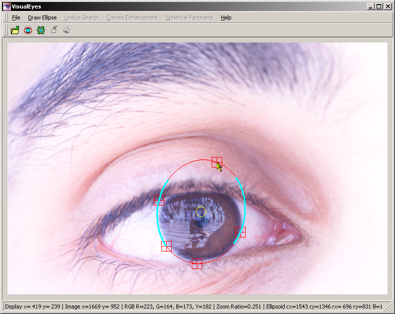
2.2.1 Points mode
You can change to points mode by selecting Draw Ellipse→Ellipse Mode: Points in the menu bar. The default is parameters mode which is explained next. In this mode, five red boxes are drawn on the arc of the ellipse and a yellow circle will appear at the center of the ellipse. By left clicking and dragging the yellow circle, you can translate the ellipse. The centers of the red boxes are the control points of the ellipse. By left clicking and dragging any of these boxes, you can change its location. The ellipse parameters will be recalculated and redrawn given the current control point locations.
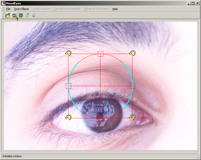
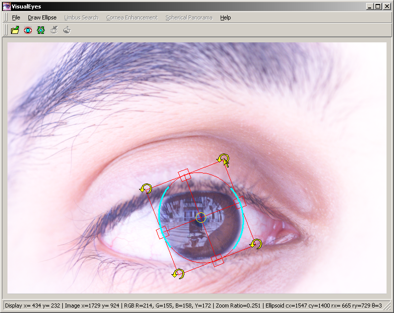
2.2.2 Parameters mode
You can change to parameters mode by selecting Draw Ellipse→Ellipse Mode: Parameters in the menu bar. The default is parameters mode. In this mode, you can modify the ellipse by directly manipulating its parameters: radii, center and tilt. The bounding box of the ellipse will be drawn in red, and a red box is drawn at the middle of each edge of this bounding box. You can left click and drag any of these small red boxes to change its location along the red line joining two of the boxes on opposite sides of the bounding box. This allows you to change the two radii of the ellipse. Also, yellow handles are drawn at the corners of the bounding box. By left clicking and dragging any of these four yellow corner handles, you can rotate the ellipse about its center (the yellow circle). This will modify the rotation angle of the ellipse. You can also translate the ellipse by left clicking and dragging the yellow circle at the center.
2.2.3. Fit to edges
You can also choose to automatically fit the ellipse to large gradients computed along radial directions by selecting
Draw Ellipse→Fit to Edges in the menu bar. This will find zero-crossings of a Laplacian filter applied in radial directions and estimate the ellipse parameters that fit those points. Note that the program finds edges within the currently set arc range. In order to set this arc range see
2.3. Set arc range. Since this is a one shot fitting using the detected edges (rather than an iterative least square fitting as the automatic limbus localization explained is in
3) it is not very reliable. If false edges are found in the cornea or sclera, the ellipse fit can be erroneous. If the localized ellipse is significantly off the limbus, you can undo it by selecting
Draw Ellipse→Undo in the menu bar. Also, for these reasons, it is recommended to run the following automatic limbus localization algorithm afterwards, even when the
fit to edges estimate seems feasible.
2.3. Set arc range
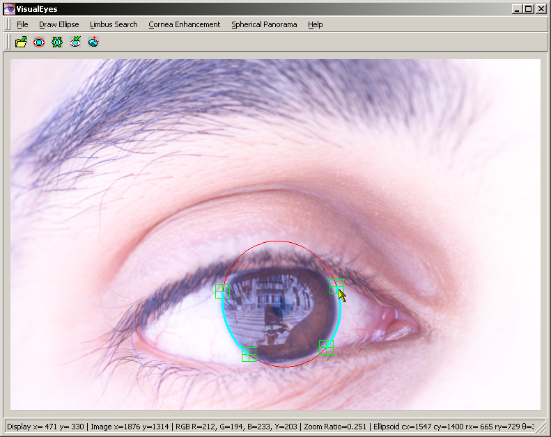
To avoid large gradients induced by non-limbus features, e.g. eyelids, being misinterpreted as the limbus in the following automatic limbus localization algorithm, its range of evaluation has to be specified in terms of the arc range of the ellipse. The current (or default if you have not already changed) arc range is drawn in cyan in both points and parameters modes. By selecting
Draw Ellipse→Ellipse Mode: Arc Range in the menu bar or by left clicking

you can modify the arc range. In this mode, four green boxes on the ends of the current arc range (cyan arcs) will be drawn. By left clicking and dragging each of these green boxes, you can change the position and hence the length of the arcs. Note that the arc range is divided into two arcs. This way it is easier to discard both upper and lower eyelids.
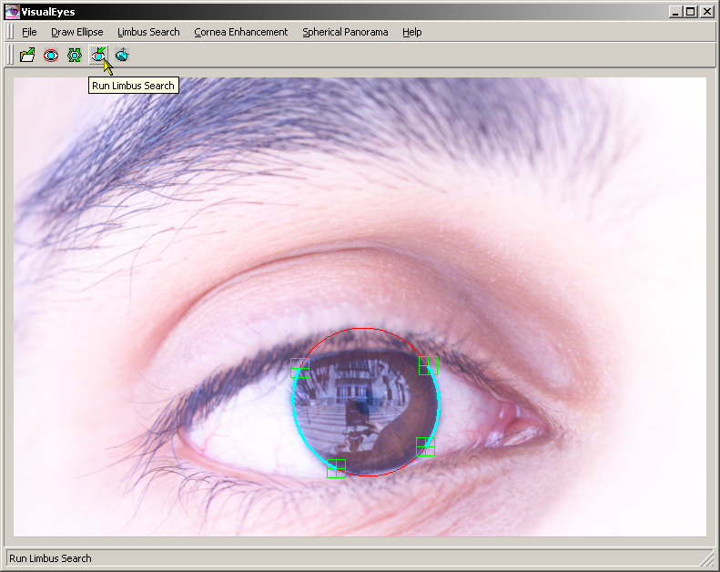
3. Automatic limbus localization
The next step is to run the automatic limbus localization algorithm which iteratively searches for the limbus parameters that best fit the gradients computed along the radial directions. The algorithm starts with the initial ellipse drawn by the user (
2.1. and
2.2.) and evaluates the gradient along the radial directions in the specified arc range (
2.3.). To run the fitting algorithm, simply select
Limbus Search→Run in the menu bar or click

.
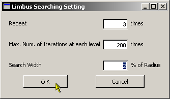
The algorithm works in a coarse to fine manner for speed up. This means that the arc of the ellipse will be evaluated sparsely in the beginning and after it converges at one level, it will evaluate the arc more densely in the next level. It switches to the next level when it converges or after the maximum number of iterations (default 200 times) is reached. In order to avoid getting trapped into a local minima, the algorithm repeats this coarse to fine iterations N times, where N can be specified in the dialog box which appears by selecting
Limbus Search→Setting in the menu bar (default N=2). You can also specify the maximum number of iterations at each level in this dialog box. Search Width in this dialog box indicates the search range along the radial direction. The default is plus minus 2% of the radius of the current ellipse.
If the ellipse after convergence does not seem to fit the limbus correctly, you can manually re-modify the ellipse and re-run the automatic limbus localization algorithm. You can go back to each of the steps in
2.2. and
2.3. by using
and
or the corresponding entries in
Draw Ellipse→Ellipse Mode in the menu bar.
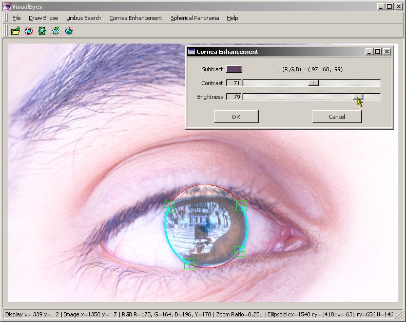
4. Image enhancement
Once the limbus in the image is localized, you can enhance the image quality of the cornea by selecting Image Enhancement→Apply in the menu bar. This will show a dialog box. You can select a color to be extracted from the pixel values within the cornea by clicking the color button (it will pop up a color selection dialog box). In many cases, you can simply use the pipette tool and select the darkest point in the cornea which well represents the iris color. Also, you can stretch or compress the contrast and brightness of the pixels in the cornea by using the slide bars in the bottom half of the dialog box. Results will be directly reflected in the image in the main pane. You can undo by selecting Image Enhancement→Undo in the menu bar.
You can save the fitting results by selecting File→Save Project. You can reload this .eye file anytime later by selecting File→Open Project and start from there.
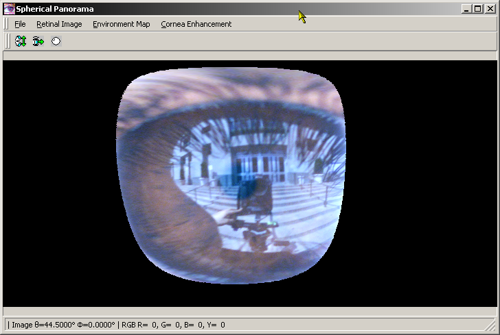
5. Spherical panorama computation
Once the limbus is localized in the image, you can compute a spherical panorama, retinal image or an spherical environment map of the surrounding environment. Although the retinal image and the spherical environment map are directly computed from the original image, in order to visually resolve the two-way ambiguity of the corneal orientation, you first need to compute a spherical panorama.
A spherical panorama will be computed by selecting
Spherical Panorama→Compute in the menu bar or by clicking

. In order to specify the parameters for computing the spherical panorama, select
Spherical Panorama→Setting in the menu bar. This will open a dialog box in which you can set the following.
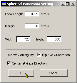
[Focal Length]
The focal length of the camera (in pixels)
[Margin]
The margin of the limbus to be discarded (in pixels) (You can discard a certain width of the cornea boundary with this. Since the limbus is a fuzzy boundary which has mixed colors of the sclera and the corneal reflection, usually this helps to discard whitish boundaries in the resulting spherical panorama.)
[Width and Height]
The width and height of the spherical panorama. (Since the spherical panorama spans 360 degrees in the horizontal direction and 180 degrees in the vertical direction, you should specify width=2*height to maintain 1:1 aspect ratio.)
[Two-way Ambiguity]
You can specify whether to flip the sign of the estimated tilt angle of the cornea with respect to the image plane computed from the estimated limbus parameters (two corneas looking at opposite directions with the same amount of tilt with respect to the image plane will produce the same ellipse in the image). You will need to check the computed spherical panorama or retinal image to see whether it should be flipped or not. For this reason, you can reset this using the icon ( ) in the computed Spherical Panorama frame (see below).
[Center at Gaze Direction]
You can specify whether or not to compute the spherical panorama with its center pointing to the direction in which the gaze direction (approximated by the optical axis of the cornea) is pointing.
Once you compute the spherical panorama by selecting
Spherical Panorama→Compute in the menu bar or by clicking
, a spherical panorama will appear in a new frame. In this frame, by clicking
, you can toggle the aforementioned flip command. If the computed retinal images (see
6.) seem to be distorted, try flipping the computed orientation of the cornea by clicking this icon.
By selecting File→Save As in the menu bar of the Spherical Panorama frame, you can save the spherical panorama as a BMP image file. Also, by selecting File→Background Color you can change the background color of the spherical panorama.
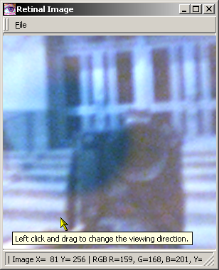
6. Retinal image computation
By left clicking any point in the spherical panorama, a retinal image (perspective image) centered around the point you clicked will appear in a new frame. By right clicking anywhere in the spherical panorama or by clicking

, a foveated retinal image (retinal image centered around the gaze direction) will appear in a new frame.
By selecting Retinal Image→Setting in the menu bar of the Spherical Panorama frame, you can specify the parameters for computing the retinal image. This will pop up a dialog box, in which you can specify the following.
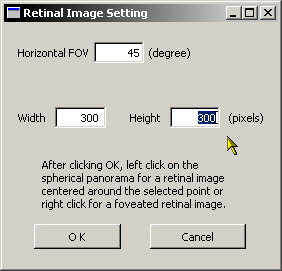
[Horizontal FOV]
The horizontal field of view in degrees.
[Width] and [Height]
The image width and height in pixels.
By left clicking and dragging the mouse cursor in the computed retinal image, you can change the viewing direction.
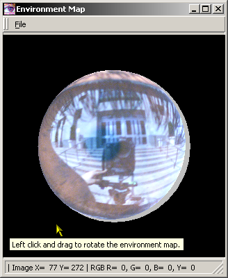
7. Spherical environment map computation
By holding SHIFT and left clicking any point in the spherical panorama, a spherical environment map with its projected center aligned to the direction of the point you clicked will appear in a new frame. By holding SHIFT and right clicking anywhere in the spherical panorama or by clicking

, a spherical environment map with its projected center aligned to the gaze direction will appear in a new frame.
By selecting Environment Map→Setting in the menu bar of the Spherical Panorama frame, you can change the size of the spherical environment map. This will pop up a dialog box in which you can specify the following.
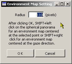
[Radius]
The radius of the spherical environment map in pixels. The size of the image will be automatically computed from the specified radius.
By left clicking and dragging the mouse cursor in the computed spherical environment map image, you can rotate the spherical environment map.
By selecting File→Save As in the menu bar of the Environment Map frame, you can save the rendered spherical environment map as a BMP image. Also, by selecting File→Background Color, you can change the background color of the image. Similarly, by selecting File→Sphere Color, you can change the color of the sphere.