


We turn attention here to the issue of biased measurement noise in the EKF and how it relates to representation of object structure.
We have assumed that features are identified in the first frame and
that measurements are obtained by comparing new images to the previous
images and that our measurements are zero-mean or very close to
zero-mean. This thinking leads to the ![]() description of
structure given earlier in
which the single unknown depth for each feature fully describes
structure. These parameters can be computed very effectively using
the EKF, which assumes zero-mean measurements.
description of
structure given earlier in
which the single unknown depth for each feature fully describes
structure. These parameters can be computed very effectively using
the EKF, which assumes zero-mean measurements.
It is common to use Kalman filters even when measurements are not truly zero-mean. Good results can be obtained if the biases are small. However, if the measurements are biased a great deal, results may be inaccurate. In the case of large biases, the biases are observable in the measurements and can therefore be estimated by augmenting the state vector with additional parameters representing the biases of the measurements. In this way, the Kalman filter can in principle be used to estimate biases in all the measurements.
However, there is a tradeoff between the accuracy that might be gained by estimating bias and the stability of the filter, which is reduced when the state vector is enlarged. When the biases are large, i.e. compared to the standard deviation of the noise, they can be estimated and can contribute to increased accuracy. But if the biases are small, they cannot be accurately estimated and they do not affect accuracy much. Thus, it is only worth augmenting the state vector to account for biases when the biases are known to be significant relative to the noise variance.
In the SfM problem, augmenting the state vector to account for bias adds two additional parameters per feature. This results in a geometry representation having a total of 7+3N parameters. Although we do not recommend this level of state augmentation, it is interesting because it can be related to the large state vector used in [10,42] and others, where each structure point is represented using three free parameters (X,Y,Z).
If we add noise bias parameters (bu,bv),
Equation 14 can be written
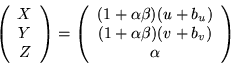 |
(20) |
It is clear that, in general, uncertainty in ![]() trivializes
uncertainty in the direction of the biases. By using initial error
variance on
trivializes
uncertainty in the direction of the biases. By using initial error
variance on ![]() that is high in comparison to the error variances
on (bu,bv), the state space is essentially reduced because the
system responds more stiffly in the direction of the biases, favoring
instead to correct the depths. In the limit (zero-mean-error
tracking) the biases can be removed completely, resulting in the
strictly lower dimensional formulation that we typically use in this
paper. Our experimental results
demonstrate that bias is indeed a second-order effect and is
justifiably ignored in most cases.
that is high in comparison to the error variances
on (bu,bv), the state space is essentially reduced because the
system responds more stiffly in the direction of the biases, favoring
instead to correct the depths. In the limit (zero-mean-error
tracking) the biases can be removed completely, resulting in the
strictly lower dimensional formulation that we typically use in this
paper. Our experimental results
demonstrate that bias is indeed a second-order effect and is
justifiably ignored in most cases.