MACHINE LEARNING February
12, 2010
COMS 4771
HOMEWORK #2
PROF. TONY JEBARA
|
DUE |
MARCH 2, 2010 BEFORE CLASS |
Instructions
1. Put everything you need to submit (matlab code, figures, writeup etc) in a folder.
2. change to that directory and create a tar ball named
For example:
joe1234@knu:~/temp1/hw2$ tar -cvf joe1234.tar *
hw2.txt
prob1.m
This would create joe1234.tar which has the all the files in the folder hw2.
3. zip the tar ball
For exampe:
joe1234@knu:~/temp1/hw2$ gzip joe1234.tar
This gives a file named joe1234.tar.gz
4. Log on to courseworks.columbia.edu
5. Go to 4771 course
6. Click on the Class Files link from the menu on the left.
7. Click on postfile
8. Upload your
9. From the drop down menu, select HWi (i=2,3,4) for homework i (in the shared files section)
10. Press the submit button
11. You can see the status of your post by clicking on Log.
PS : These files can not be seen by other students. Do not worry about it.
Your write-up should be in ASCII plain text format (.txt) or Postscipt (.ps) or
the Adobe Portable Document Format (.pdf). Please do not submit Microsoft
Office documents, LaTeX source code, or something more exotic. We will not be
able to read it. LaTeX is preferred and highly recommended, but it is not
mandatory. You can use any document editing software you wish, as long as the
final product is in .ps or .pdf. Even if you do not use LaTeX to prepare your
document, you can use LaTeX notation to mark up complicated mathematical
expressions, for example, in comments in your Matlab code. See the “Tutorials”
page for more information on LaTeX.. All your code
should be written in Matlab. Please submit all your souce files, each function
in a separate file. Clearly denote what each function does, which problem it
belongs to, and what the inputs and the outputs are. Do not resubmit code or
data provided to you. Do not submit code written by others. Identical
submissions will be detected and both parties will get zero credit. Shorter
code is better. Sample code is available on the “Tutorials” web page. Datasets
are available from the “Handouts” web page.
You may include figures directly in your write-up or include them separately as
.jpg, .gif, .ps or .eps files, and refer to them by filename. Submit work via courseworks.columbia.edu.
If something goes wrong, ask the TA's for help. Thanks.
1.
(10 points) Support Vector Machines: Assume we have trained 3
separable support vector machines on the 2D data (the axes go from –1 to 1 in
both horizontal and vertical direction) using 3 different kernels as follows:
(a)
a linear kernel (i.e. the standard linear SVM):
![]()
(b)
a quadratic polynomial kernel:

(c)
an RBF kernel:

Assume
we now translate the data by adding a large constant value (i.e. 10) to the
vertical coordinate of each of the data points, i.e. a point (x1,x2) becomes (x1,x2+10)
If we
retrain the above SVMs on this new data, do the resulting SVM boundary for
change relative to the data points? Say if it does change or not for case (a),
case (b) and case (c). Briefly explain why or why not it changes for all 3 cases (a), (b) and (c) and suggest or draw what
happens to the resulting new boundaries when appropriate.
2.
(10 points) VC Dimension: Assume we are forming a two-dimensional
classifier in the space:

a)
Instead of the usual linear classifier, consider the following circular
classifier in 2d:
![]()
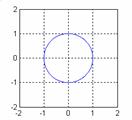
Here,
the parameter of the classifier is b, just a scalar. What is the VC dimension h
of this quadratic classifier in two dimensional classification problems? Explain
how you came up with a number for h by drawing examples. Draw a good
configuration of the h points where the quadratic classifier is able to
shatter perfectly and show the quadratic decision for all 2h
binary labelings of the points. Also draw a poor configuration for h
points that the quadratic classifier cannot shatter and show the particular
labelings of the points that it cannot shatter. By ‘shatter’ we mean that the
quadratic classifier will perfectly separate the data despite an arbitrary binary
labeling of the points.
b)
Now consider another circular classifier in 2d and do the same as above.
![]()
Here,
the parameters of the classifier are a and b, which
are both just scalars. HINT: think about what happens when a goes negative!
3. (30
points) SVM on Image Data:
Build an
SVM from Steve Gunn’s code to classify the data in shoesducks.mat. These are
images of shoes and ducks that you want to build a classifier for. Note: you
can find Steve Gunn’s Matlab code for SVMs here:
http://www.isis.ecs.soton.ac.uk/resources/svminfo/
In svc.m replace
[alpha
lambda how] = qp(…);
with
[alpha
lambda how] = quadprog(H,c,[],[],A,b,vlb,vub,x0);
Clearly
denote the various components and the function calls or scripts that execute
your Matlab functions. Shorter code is better. Note, to save the current figure
in Matlab as a postscript file you can type:
print –depsc filename.eps
Sample
code is available on the “Tutorials” web page. Datasets are available from the
“Handouts” web page. Extract the support vector machine code from Steve Gunn’s
GUI. This should let you easily learn a classifier with kernels with the
decision boundary being represented as follows:
![]()
Refer to
the Gunn’s code and Burges’ tutorial for more details.
To test
your SVM, you will build a simple object recognition system. Download the
images given in from shoesducks.mat. This loads a
matrix X of size 144 by 768 and a vector Y of size 144 by 1. The X matrix
contains 144 images, each is a vector of length 768.
These vectors are not quite images but rather are the contour profile of the
top part of the object (either a shoe or a duck). To view them as contours,
just type plot(X(4,:)) which will plot a contour of
the 4th object (a duck in this case with Y(4) being 1). There are a
total of 72 images of ducks and 72 images of shoes at different 3D rotations.
Train your SVM on the half of the examples and test on the other half (or other
subsets of the examples as you see fit). Show performance of the SVM for
linear, polynomial and RBF kernels with different settings of the polynomial order,
sigma and C value. Try to hunt for a good setting of these parameters to obtain
high recognition accuracy.
(BONUS)
Bonus question has been cancelled.