Towards a Mechanical Music Transcriber
by
Terrence J. Truta
Introduction
Many musicians buy music transcripts for popular songs because they don't have the ability to identify musical notes by ear. Somewhat paradoxically only very few musicians have this skill.* If an individual with this skill isn't available, transcriptions of recorded music are made tediously by trial and error, slowing music down, asking the original musicians (if available), or some combination of these things. Clearly a mechanical music transcriber would be a great aid to people who wish to transcribe music.
A music transcriber, whether mechanical or human, records the pitch and duration of various musical notes. In addition, a music transcriber identifies the beat of a piece of music. Using machine learning to identify the pitch of a music note would be a first step towards building a full-featured music transcriber.
This paper describes neural networks that are trained to classify audio signals in the form of musical notes. In particular, the neural networks are trained to classify monophonic sound (i.e. one note played at a time) as opposed to polyphonic sound (i.e. where there are multiple notes played at once).
Approach
I used sampled data as input to a neural network. To get this data, I modified a Java library package called SoundBite to generate audio data that represented audio waves of different pitches. A sine wave's frequency was varied to generate the 12 different pitches of the western scale. In total 36 different sound waves were created (3 of each pitch) which spans 3 octaves of the western scale. The amplitude remained fixed.
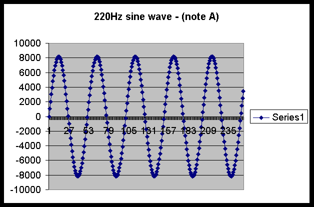
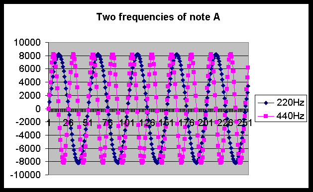
I used an 11025 samples/second rate to generate the wave. This means that 11025 different integer values make up one second of sound. However, the frequency of the lowest music note was 220 Hz. This means that one complete cycle at this pitch is represented with about 50 integer values. Given this amount of repetition, I decided that all 11025 integer values weren't needed as inputs to the neural network. I varied the amount of the samples used as inputs to the neural network. I used 255 (about 5 cycles of 220Hz), 26 (about 1/2 cycle), and 12 (about 1/4 cycle) samples as input in different experiments. Figure 1 shows one training example with 255 integers graphically. Each dot on the graph corresponds to an integer value. Figure 2 shows this same training example along with another example that has twice the frequency (one octave higher) and thus should be classified as the same note.
FIGURE 1
FIGURE 2
I adapted the neural network code used in project 3 to read in and learn the sampled audio data. The audio data for each example like the image data was stored in file. Nevertheless I needed to write new routines to read in the data. In addition, several other functions were rewritten and/or renamed to process the audio data such as load_target() and load_input_with_image().
Experiments
For my first experiment, I trained a network with 255 inputs and 12 outputs. The inputs as mentioned above are integer values ranging from 8000 to -8000. The 12 outputs correspond to the 12 tones in the western music chromatic scale (A, A#, G, etc). If the 255 inputs represent a sound wave of 220Hz, 440Hz, or 880Hz (all corresponding to the note A) then the first network output should be on and the other 11 off. Similarly the second unit should be on only if a sound wave that represents an A# is loaded in the inputs. I varied the number of hidden units between 12, 24, and 36 and also varied the learning rate.
Initially I was just concerned about having the neural network learn a hypothesis that fit the training examples so I didn't use a separate validation or testing set. I pondered if this break from the traditional accepted methods of experimenting was warranted. My view is that if a neural network can learn to correctly classify 3 octaves of sine wave frequency then it can be used as is in a monophonic transcription system. Since the motivation for this experiment is to move toward this goal, the end justifies the means. In addition, it isn't clear what examples should be in the validation set and testing set. Two candidates are a different set of frequencies (for example where A is 110Hz) and the same set of frequencies made up of different timbres (for example a piano wave form instead of a sine wave form).
For the next experiment I tried to train a neural network to recognize a particular note. For example, an A recognizer would have one output port and it would be on if the a sound wave that represents an A is loaded into the input units. In addition, to using 255 input units, I tried using 26 and 12 input units. I arrived at these numbers since it allowed for 1/2 and 1/4 of a cycle respectively to be represented for the slowest frequency in the training examples (220Hz). The motivation for this was that I wasn't having much success with the neural networks with 255 input units and I hypothesized that fewer units would be easier to train. In addition, I also tried many experiments with the same frequencies but a much lower amplitude. These integer samples of these examples oscillated between around 300 and -300.
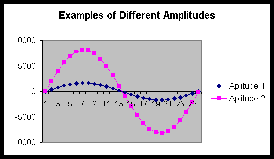
Success again proved elusive and thus I tried a new learning task that I thought might work. This time I tried to train a neural network to recognize amplitude. I used the modified SoundBite package to generate 12 different amplitude examples to get the data. Two different examples are plotted in Figure 3.
For reasons I will explain later in this paper, I also repeated many of the experiments with a modified squashing function. I added the constant 0.0001 to the following modified sigmoid function:
(1.0 / (1.0 + exp(-x*0.0001)))
This had the effect of reducing the steepness of the sigmoid curve.
FIGURE 3
Results
The results are not encouraging. For the first experiment with 255 inputs and 12 outputs, it achieved a whopping 0% accuracy rate on the training examples after 5000 epochs regardless of the number of hidden units or learning rate values. For the next experiment, an A recognizer achieved a 100% accuracy over the training examples. This was achieved with a 26x24x1 network with learning rate set to 3.0 after 73 epochs. I thought that this was a breakthrough but I was unable to get similar results from other single note recognizers (i.e. A#, G, G#, etc). All other single note recognizers received only a 91.6667% accuracy, which is the baseline since only 12 examples were used to train. The 91.6667% baseline was not exceeded either with the amplitude recognizer experiments.
After a few unsuccessful attempts at learning the pitch of sampled audio data I began to think that the problem wasn't formulated correctly. It may be the case that the temporal aspect of sampled audio data by be hindering the learning ability of the neural network. This makes some sense because with data from an audio wave, the values of the inputs don't matter as much as how far away one wave peek is from another wave peek. Using weights on input units which determine how much a particular unit matters to a correct output. Its hard to intuitively understand how the weights of a neural network can encode frequency recognition. However amplitude recognition seemed more doable since the values of the inputs actually correspond directly to the correct target function.
After I failed to have success on an amplitude recognizer I decided something may be wrong with the code I modified. After exhaustive debugging I found a potential problem. The squashing function wasn't doing its job correctly. On my PC using Microsoft c++ 5.0, the sigmoid function rounded up and outputted a 1.0 for any inputted value over 21. While learning audio samples the values inputted into a sigmoid are sometimes as high as 30000 since each of the 255 input values can range between -9000 and 9000. This was a problem because in the function bpnn_hidden_error the following line computes how much the hidden unit should be changed:
delta_h[j] = h * (1.0 - h) * sum;
h is the value of a hidden unit (the value of h changes inside a loop to compute each hidden unit change). Since h was sometimes mistakenly 1.0, delta h is 0. Thus the often the total hidden error sum was 0. The hidden weights were never changed since backprop mistakenly believed that the weights were perfect. Only the weights leading to the output unit were being changed.
How can a neural network learn well if the hidden units aren't updated? In order to try to get around this I changed the sigmoid function a little. I added the constant 0.0001 as I mentioned above. This had the effect of reducing the steepness of the sigmoid curve. Now a value of 30000 has the value 0.952574 instead of 1.0. Unfortunately, this new squashing function still didn't do its job since sometimes the sum was many factors of ten greater than 30000. Thus this change didn't help to improve the accuracy
For my next workaround, I tried to regenerating the data using a much smaller amplitude. Recall originally that the amplitude ranged from around 8000 to -8000. The new data had an amplitude that ranged from around 300 to -300. I hypothesized that this might work since the neural network package worked fine with image data that I believe had a somewhat similar range of integer values of 0 to 255. However, the squashing function still often outputted a 1.0 and thus caused the total hidden error to be 0.
The perplexing mystery of the squashing function remains to be solved. I believe that there may be a bug that I introduced into the code when I converted the package from an image classifier to an audio classifier. However, I have exhaustively searched for any bugs in the code and have found none.
Related Work
The approach I took for my experiments to learn audio frequencies differs from some recent approaches [1,2] which preprocesses the audio wave to obtain a frequency representation of wave. Fortunately for those in the machine learning community interested in music transcription, these approaches work very well according to the researchers doing the work. My diverging approach was not by choice. Firstly, I wasn't aware of previous work in this area when I conceived the idea for this experiment and started to work on it. Secondly, I was unable to find enough information about using preprocessing techniques to be able to use them.
In ``Note Recognition in Polyphonic Music using Neural Networks,''[1] Shuttleworth and Wilson provide an introduction of the issues associated with mechanical music transcription. They focus particularly with the difficulty classifying polyphonic sounds and how the Multiresolution Fourier Transform is better than other popular signal representations to use as input to a neural network (interestingly the authors don't even mention my approach of using raw sampled data as input). The authors also mention the current approaches being done to recognize the beat of the music being transcribed. Not only is a beat classifier part of a complete music transcriber, it can also reduce the amount of data the system needs to handle since musical events such as the on-set of new notes very often occur on a beat. The paper finishes with a discussion of other approaches to musical transcription and current research areas. One research area is using Hidden Markov Models, which are commonly used for speech processing, to help incorporate the temporal aspects of music into musical transcription.
Duncan Thomson in "A Connectionist System for Instrument and Pitch Discrimination"[2], describes the research he is doing into music transcription and the human hearing process. He too is using a neural network. In his system, sounds are preprocessed ("analyzed by performing constant Q transforms on slices at constant intervals", whatever that means). The sound representations are fed into the neural network. The output of the neural network includes the note played and instrument that played it. His conclusion states that his system performs pitch and timbre recognition very well and therefore his system can be used as a platform to build a music transcription system.
Chan and Stolfo in "A Comparative Evaluation of Voting and Meta-learning on Partitioned Data" first explain the need to partition data archives. It is because some databases are too big to fit into main memory and many learning algorithms require the data to fit there. Partitioning data is one solution. The issue with partitioning data is to maintain accuracy. The authors show how meta-learning partitioned data achieves better results than polling multiple classifiers and using the most popular classification. The paper details two methods for meta-learning partitioned data. One method which they call a combiner approach seems to be synonymous with stacked generalization. The other approach is the arbiter method, which involves training a separate classifier on examples that the two base classifiers don't agree on. The authors go on to mention how a construct called an arbiter tree can be used to meta-learn multiple classifiers with favorable results.
Conclusions
References