Maximum Entropy Discrimination Mixtures of Gaussians (Medmix)

Software

Results

Nonstationary Kernel Selection

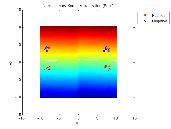
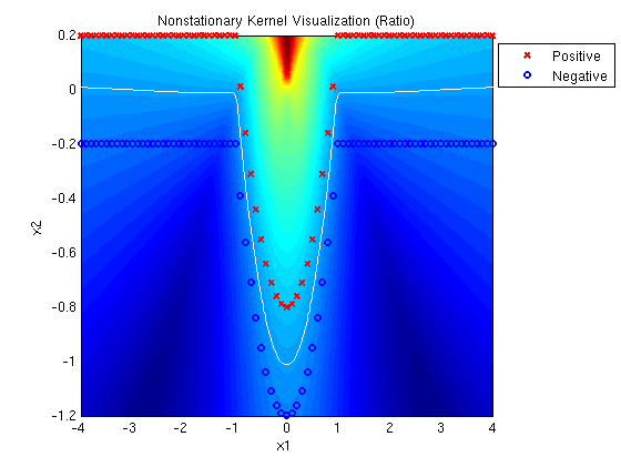
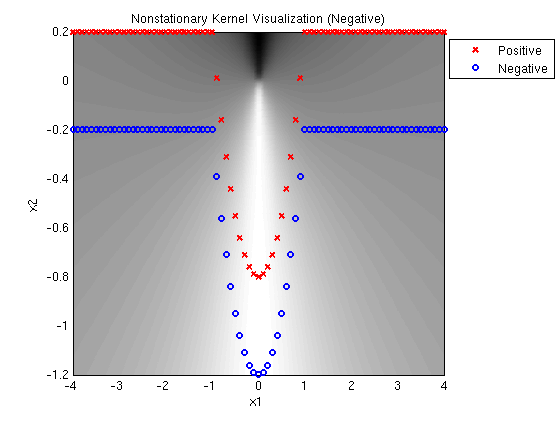
• This visualization uses synthetic data to illustrate the idea of nonstationary kernel selection. We chose 162 examples at regular intervals along a function that is part linear and part quadratic. Positive examples are translated 0.2 along the vertical axis and negative examples are translated in the oppostite direction.

  A MED mixture of Gaussians with one linear and one quadratic kernel determines the following decision surface, which clearly illustrates the linear and quadratic components. Note that the solution has large margin and cannot be accomplished with a linear combination of a linear and quadratic kernel.
  

  The convergence of MED from a random initialization can be seen in this AVI movie.
  
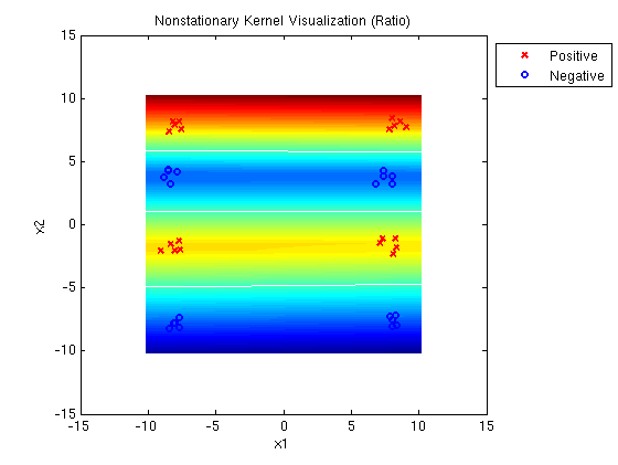
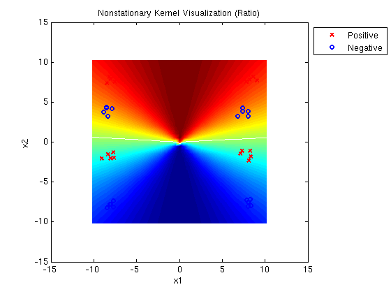
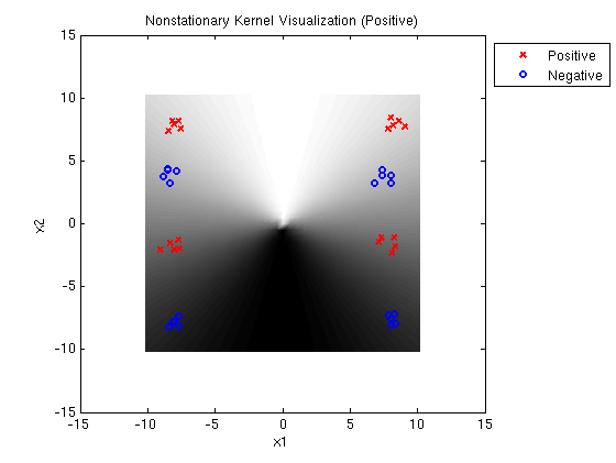
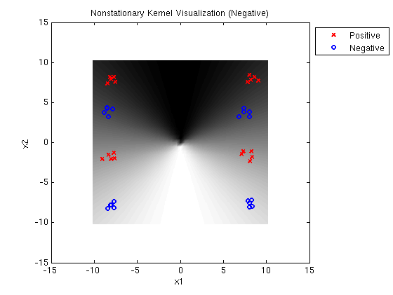
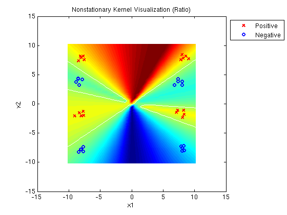
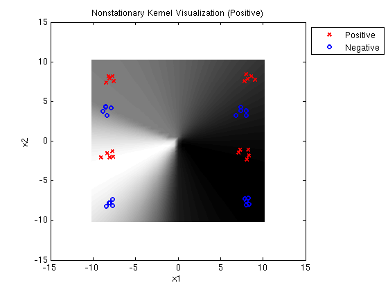
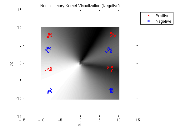
  Linear-Quadratic MED ratio:
  

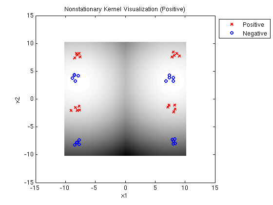
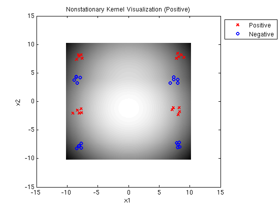
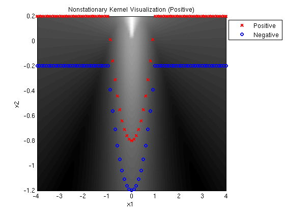
  Linear-Quadratic MED positive:
  

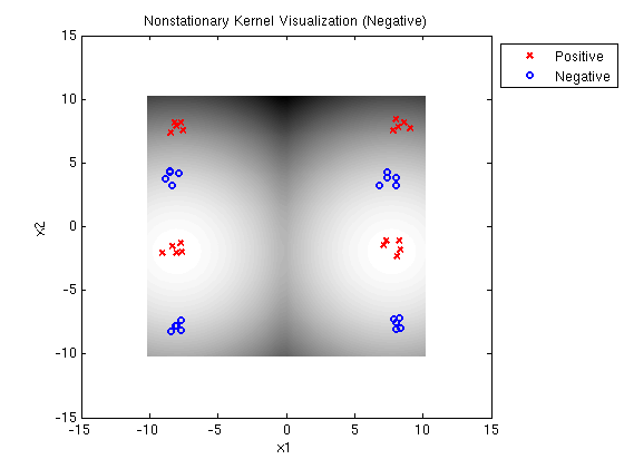
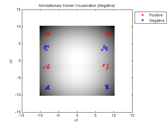
  Linear-Quadratic MED negative:
  

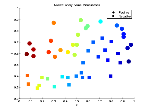
• Following is a plot of data that were generated from a linear and a quadratic kernel with added noise. Circles represent positive examples. Squares represent negative examples. Shading indicates mixing between the linear and quadtratic kernels at each input example when the technique is applied for classification. (Red indicates linear kernel; Blue indicates quadratic kernel.)
  

Large Margin Ratio of Gaussian Mixtures

This visualization uses synthetic data to illustrate the idea of large margin discrimination using a ratio of mixture models. We chose 40 examples from eight Gaussian clusters that are interleaved vertically with respect to class label. This example is extreme, because, in effect, a variable has been introduced that has no bearing on correct classification. We use a ratio of two mixture models, each with two identity covariance Gaussian components per class, to classify the data.

• When we train the model using maximum likelihood, the misfit between the model and the observed data becomes problematic. Maximum likelihood parameter estimation places the Gaussian means in the midst of a cluster of data from the opposite class. This results in 50-50 classification accuracy.
  

  Eight Gaussians ML ratio:
  

  Eight Gaussians ML positive:
  

  Eight Gaussians ML negative:
  
  
  

• When we train the model using MED parameter estimation, the classification performance drives the parameters toward a more discriminative setting. Though this example is extreme, it is not irrelevant. There are many discriminative settings in which the data do not exactly fit the model.

  Eight Gaussians MED ratio:
  

  Eight Gaussians MED positive:
  

  Eight Gaussians MED negative:
  

• When the kernels (all linear) are normalized, the results are similar. The normalization rescales the axes and produces the following:

  Eight Gaussians ML ratio (normalized kernels):
  

  Eight Gaussians ML positive (normalized kernels):
  

  Eight Gaussians ML negative (normalized kernels):
  

  Eight Gaussians MED ratio (normalized kernels):
  

  Eight Gaussians MED positive (normalized kernels):
  

  Eight Gaussians MED negative (normalized kernels):
  
  
  

• It is important to note that unlike the SDP kernel combination, the MED kernel mixture can fall into local minima. Different random initializations can result in qualitatively different solutions. To address this, we use multiple restarts and a model is chosen based on the objective.

• The flexibility of the ratio of mixture models is far greater than that of the SVM. We can vary the number of mixture components for each class, and the space in which the component distributions are projected. Whereas the SDP kernel combination does not benefit by using each kernel more than once, the MED kernel mixture does benefit.

Iterative optimizer

• Complete table of results from timing experiment with the improved code.

• A plot of timing trends: